In my last posts, I analysed the significance of experience for different occupational groups. In this post, I will turn the interest towards education. I will again start with engineers and see if I can expand my analysis to all occupational groups.
First, define libraries and functions.
library (tidyverse) ## -- Attaching packages ------------------------------------------- tidyverse 1.2.1 --## v ggplot2 3.2.0 v purrr 0.3.2
## v tibble 2.1.3 v dplyr 0.8.3
## v tidyr 0.8.3 v stringr 1.4.0
## v readr 1.3.1 v forcats 0.4.0## -- Conflicts ---------------------------------------------- tidyverse_conflicts() --
## x dplyr::filter() masks stats::filter()
## x dplyr::lag() masks stats::lag()library (broom)
library (car)## Loading required package: carData##
## Attaching package: 'car'## The following object is masked from 'package:dplyr':
##
## recode## The following object is masked from 'package:purrr':
##
## somelibrary (splines)
#install_github("ZheyuanLi/SplinesUtils")
library(SplinesUtils)
readfile <- function (file1){
read_csv (file1, col_types = cols(), locale = readr::locale (encoding = "latin1"), na = c("..", "NA")) %>%
gather (starts_with("19"), starts_with("20"), key = "year", value = salary) %>%
drop_na() %>%
mutate (year_n = parse_number (year))
}The data table is downloaded from Statistics Sweden. It is saved as a comma-delimited file without heading, 000000CY.csv, http://www.statistikdatabasen.scb.se/pxweb/en/ssd/.
The table: Average basic salary, monthly salary and women´s salary as a percentage of men´s salary by sector, occupational group (SSYK 2012), sex and educational level (SUN). Year 2014 - 2018 Monthly salary All sectors
We expect that education is an important factor in salaries. As a null hypothesis, we assume that education is not related to the salary and examine if we can reject this hypothesis with the data from Statistics Sweden.
The column level of education is renamed because TukeyHSD doesn’t handle variable names within quotes.
tb <- readfile("000000CY.csv") %>%
  filter(`occuptional  (SSYK 2012)` == "214 Engineering professionals") %>%
  mutate(edulevel = `level of education`)

tb %>%
  ggplot () +
    geom_point (mapping = aes(x = year_n,y = salary, colour = `level of education`, shape=sex)) +
  labs(
    x = "Year",
    y = "Salary (SEK/month)"
  )
Figure 1: SSYK 214, Architects, engineers and related professionals, Year 2014 - 2018
model <- lm (log(salary) ~ year_n + sex + edulevel, data = tb)

tb <- bind_cols(tb, as_tibble(exp(predict(model, tb, interval = "confidence"))))
The F-value from the Anova table for years is 40 (Pr(>F) < 2.2e-16), sufficient for rejecting the null hypothesis that education has no effect on the salary holding year as constant. The adjusted R-squared value is 0,833 implying a good fit of the model.
tb %>%
  ggplot () +
    geom_point (mapping = aes(x = year_n,y = fit, colour = edulevel, shape = sex)) +
  labs(
    x = "Year",
    y = "Salary (SEK/month)"
  )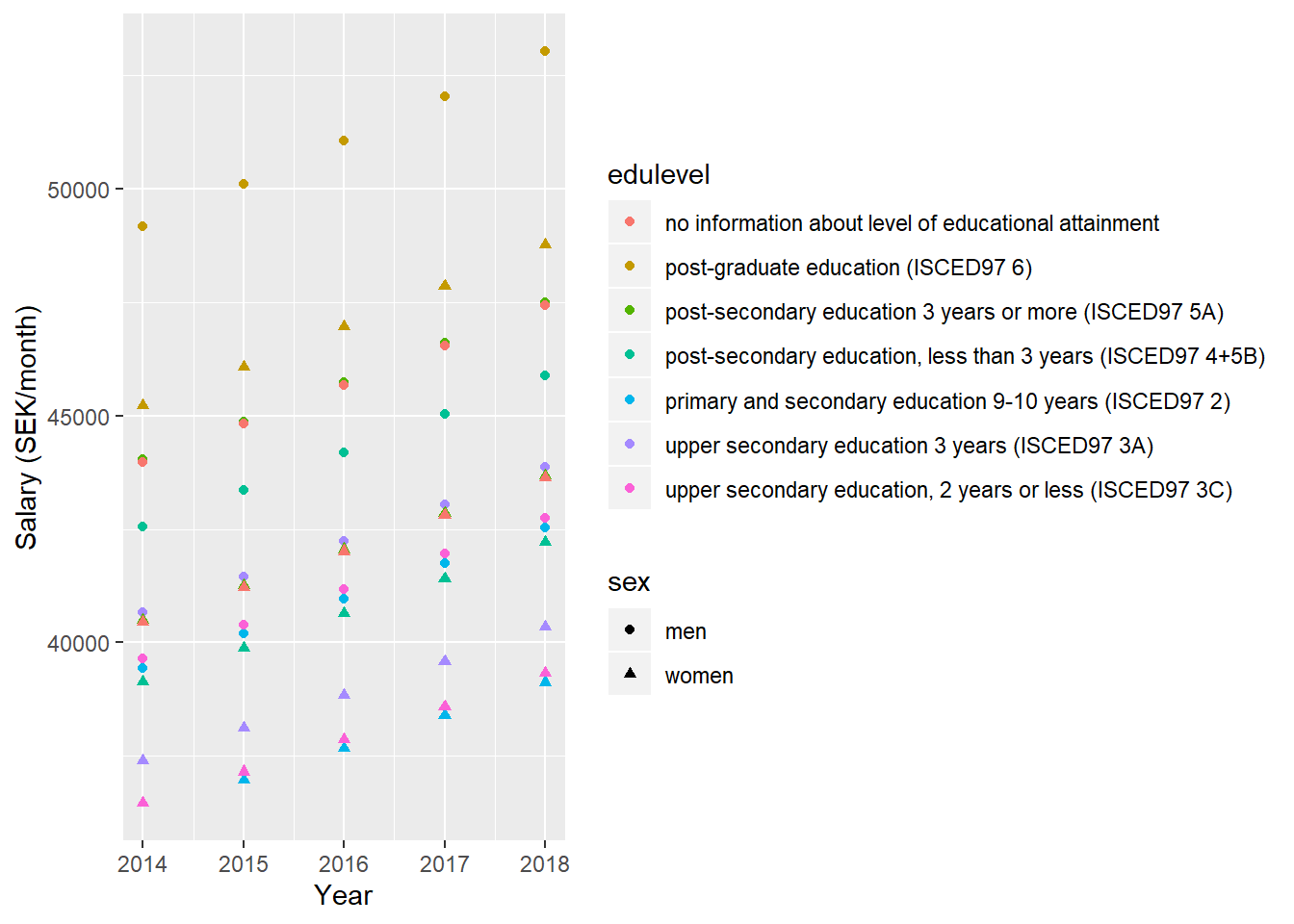
Figure 2: Model fit, SSYK 214, Architects, engineers and related professionals, Year 2014 - 2018
summary(model) %>%
  tidy() %>%
  knitr::kable(
  booktabs = TRUE,
caption = 'Summary from linear model fit')| term | estimate | std.error | statistic | p.value |
|---|---|---|---|---|
| (Intercept) | -27.3895893 | 6.6236266 | -4.1351349 | 0.0001120 |
| year_n | 0.0189082 | 0.0032856 | 5.7549246 | 0.0000003 |
| sexwomen | -0.0837412 | 0.0092178 | -9.0847619 | 0.0000000 |
| edulevelpost-graduate education (ISCED97 6) | 0.1114561 | 0.0171029 | 6.5167907 | 0.0000000 |
| edulevelpost-secondary education 3 years or more (ISCED97 5A) | 0.0010205 | 0.0171029 | 0.0596699 | 0.9526168 |
| edulevelpost-secondary education, less than 3 years (ISCED97 4+5B) | -0.0332012 | 0.0171029 | -1.9412595 | 0.0569278 |
| edulevelprimary and secondary education 9-10 years (ISCED97 2) | -0.1089810 | 0.0175947 | -6.1939725 | 0.0000001 |
| edulevelupper secondary education 3 years (ISCED97 3A) | -0.0784305 | 0.0171029 | -4.5857936 | 0.0000235 |
| edulevelupper secondary education, 2 years or less (ISCED97 3C) | -0.1040503 | 0.0171029 | -6.0837761 | 0.0000001 |
summary(model)$adj.r.squared ## [1] 0.8327314Anova(model, type = 2) %>%
tidy() %>%
knitr::kable(
booktabs = TRUE,
caption = 'Anova report from linear model fit')| term | sumsq | df | statistic | p.value |
|---|---|---|---|---|
| year_n | 0.0484384 | 1 | 33.11916 | 3e-07 |
| sex | 0.1207084 | 1 | 82.53290 | 0e+00 |
| edulevel | 0.3529225 | 6 | 40.21774 | 0e+00 |
| Residuals | 0.0877529 | 60 | NA | NA |
How much do the different levels of education affect the salary? We can calculate the differences between the levels with Tukey’s honest significant difference. All significant level differences are shown in the table below.
tukeytable <- TukeyHSD(aov(log(salary) ~ sex + edulevel, data = tb)) %>%
  tidy() %>%
  mutate(percdiff = (1 / exp(estimate) - 1) * 100)

tukeytable  %>%
  filter(adj.p.value < 0.05) %>%
  arrange(estimate) %>%
  knitr::kable(
  booktabs = TRUE,
caption = 'Tukey HSD 95 % confidence intervals for the pairwise significant differences')| term | comparison | estimate | conf.low | conf.high | adj.p.value | percdiff |
|---|---|---|---|---|---|---|
| edulevel | primary and secondary education 9-10 years (ISCED97 2)-post-graduate education (ISCED97 6) | -0.2160450 | -0.2822364 | -0.1498535 | 0.0000000 | 24.115819 |
| edulevel | upper secondary education, 2 years or less (ISCED97 3C)-post-graduate education (ISCED97 6) | -0.2155065 | -0.2799325 | -0.1510804 | 0.0000000 | 24.049001 |
| edulevel | upper secondary education 3 years (ISCED97 3A)-post-graduate education (ISCED97 6) | -0.1898866 | -0.2543126 | -0.1254606 | 0.0000000 | 20.911247 |
| edulevel | post-secondary education, less than 3 years (ISCED97 4+5B)-post-graduate education (ISCED97 6) | -0.1446573 | -0.2090834 | -0.0802313 | 0.0000001 | 15.564352 |
| edulevel | post-secondary education 3 years or more (ISCED97 5A)-post-graduate education (ISCED97 6) | -0.1104356 | -0.1748616 | -0.0460096 | 0.0000443 | 11.676444 |
| edulevel | primary and secondary education 9-10 years (ISCED97 2)-post-secondary education 3 years or more (ISCED97 5A) | -0.1056094 | -0.1718008 | -0.0394179 | 0.0001649 | 11.138763 |
| edulevel | upper secondary education, 2 years or less (ISCED97 3C)-post-secondary education 3 years or more (ISCED97 5A) | -0.1050709 | -0.1694969 | -0.0406448 | 0.0001119 | 11.078932 |
| edulevel | primary and secondary education 9-10 years (ISCED97 2)-no information about level of educational attainment | -0.1045888 | -0.1707803 | -0.0383974 | 0.0001950 | 11.025400 |
| edulevel | upper secondary education, 2 years or less (ISCED97 3C)-no information about level of educational attainment | -0.1040503 | -0.1684764 | -0.0396243 | 0.0001331 | 10.965630 |
| sex | women-men | -0.0803151 | -0.1030666 | -0.0575637 | 0.0000000 | 8.362851 |
| edulevel | upper secondary education 3 years (ISCED97 3A)-post-secondary education 3 years or more (ISCED97 5A) | -0.0794510 | -0.1438770 | -0.0150250 | 0.0066749 | 8.269249 |
| edulevel | upper secondary education 3 years (ISCED97 3A)-no information about level of educational attainment | -0.0784305 | -0.1428565 | -0.0140044 | 0.0077374 | 8.158814 |
| edulevel | primary and secondary education 9-10 years (ISCED97 2)-post-secondary education, less than 3 years (ISCED97 4+5B) | -0.0713876 | -0.1375791 | -0.0051962 | 0.0264560 | 7.399745 |
| edulevel | upper secondary education, 2 years or less (ISCED97 3C)-post-secondary education, less than 3 years (ISCED97 4+5B) | -0.0708491 | -0.1352751 | -0.0064231 | 0.0221087 | 7.341926 |
| edulevel | post-graduate education (ISCED97 6)-no information about level of educational attainment | 0.1114561 | 0.0470301 | 0.1758822 | 0.0000370 | -10.546938 |
We can conclude from the summary table that there is a positive correlation between longer education and higher salaries.
From the table of Tukey’s honest significant difference, we can see the difference in salaries between the different education lengths. Note that the estimates are negative due to the log transformation, the untransformed differences are in the column percdiff.
Can we approximate how much the salaries increase by one year of education by assigning a numeric value to the factors in the table?
As a first approach, I will use the data in the following table.
I will use a B-spline function to approximate the increase in salaries over age. The rows for “no information about the level of educational attainment” is removed from the table from Statistics Sweden.
numedulevel <- read.csv("edulevel.csv")

numedulevel %>%
  knitr::kable(
  booktabs = TRUE,
caption = 'Initial approach, length of education') | level.of.education | eduyears |
|---|---|
| primary and secondary education 9-10 years (ISCED97 2) | 9 |
| upper secondary education, 2 years or less (ISCED97 3C) | 11 |
| upper secondary education 3 years (ISCED97 3A) | 12 |
| post-secondary education, less than 3 years (ISCED97 4+5B) | 14 |
| post-secondary education 3 years or more (ISCED97 5A) | 15 |
| post-graduate education (ISCED97 6) | 19 |
| no information about level of educational attainment | NA |
tbnum <- tb %>%
    right_join(numedulevel, by = c("level of education" = "level.of.education")) %>%
  filter(!is.na(eduyears))
## Warning: Column `level of education`/`level.of.education` joining character
## vector and factor, coercing into character vectormodelcont <- lm(log(salary) ~ bs(eduyears, knots = c(14)) + year_n + sex, data = tbnum)
tbnum <- bind_cols(tbnum, as_tibble(exp(predict(modelcont, tbnum, interval = "confidence"))))The F-value from the Anova table for years is 146 and the adjusted R-squared value is 0,932 implying a good fit of the model. Both the F-value and the adjusted R-squared increased from then using the categorical predictors. (Removing the rows with “no information about level of educational attainment” improves the adjusted R-squared for the model with categorical predictors to 0.931.)
tbnum %>%
  ggplot () +
    geom_point (mapping = aes(x = year_n,y = fit1, colour = eduyears, shape = sex)) +
  labs(
    x = "Year",
    y = "Salary (SEK/month)"
  )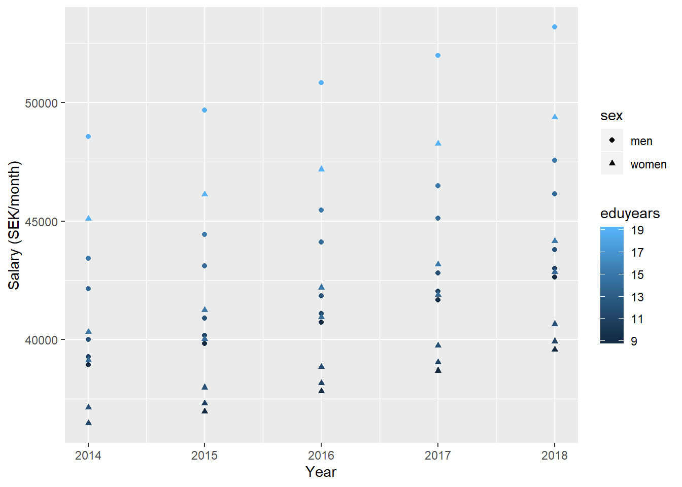
Figure 3: Model fit, SSYK 214, Architects, engineers and related professionals, Year 2014 - 2018
summary(modelcont) %>%
  tidy() %>%
  knitr::kable(
  booktabs = TRUE,
caption = 'Summary from linear model fit')| term | estimate | std.error | statistic | p.value |
|---|---|---|---|---|
| (Intercept) | -35.1115742 | 4.5503183 | -7.7162898 | 0.0000000 |
| bs(eduyears, knots = c(14))1 | -0.0113708 | 0.0237866 | -0.4780331 | 0.6346302 |
| bs(eduyears, knots = c(14))2 | 0.0719453 | 0.0468930 | 1.5342429 | 0.1310323 |
| bs(eduyears, knots = c(14))3 | 0.1850177 | 0.0567742 | 3.2588347 | 0.0019749 |
| bs(eduyears, knots = c(14))4 | 0.2212179 | 0.0111456 | 19.8480339 | 0.0000000 |
| year_n | 0.0226818 | 0.0022569 | 10.0500379 | 0.0000000 |
| sexwomen | -0.0743275 | 0.0063230 | -11.7551579 | 0.0000000 |
summary(modelcont)$adj.r.squared ## [1] 0.9316461Anova(modelcont, type = 2) %>%
tidy() %>%
knitr::kable(
booktabs = TRUE,
caption = 'Anova report from linear model fit')| term | sumsq | df | statistic | p.value |
|---|---|---|---|---|
| bs(eduyears, knots = c(14)) | 0.3429901 | 4 | 145.7866 | 0 |
| year_n | 0.0594072 | 1 | 101.0033 | 0 |
| sex | 0.0812757 | 1 | 138.1837 | 0 |
| Residuals | 0.0305849 | 52 | NA | NA |
What does the continous function from the model look like?
contspline <- RegBsplineAsPiecePoly(modelcont, "bs(eduyears, knots = c(14))")

tibble(eduyears = 9:19) %>%
  ggplot () +
    geom_point (mapping = aes(x = eduyears,y = predict(contspline, eduyears))) +
  labs(
    x = "Years of education",
    y = "Salary"
  )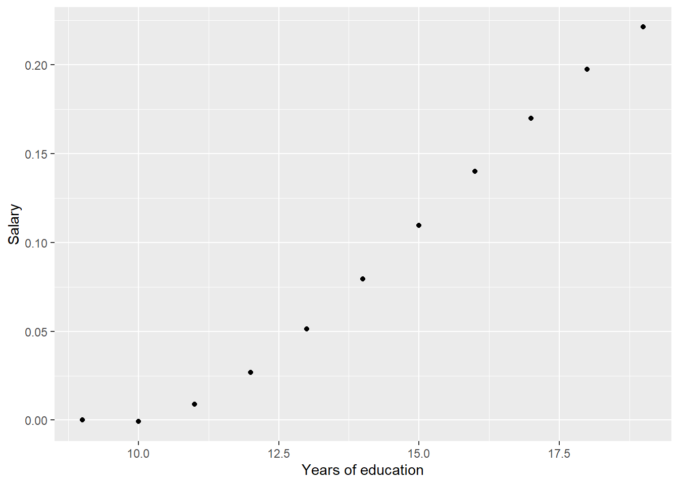
Figure 4: Model fit, SSYK 214, Correlation between education and salary
And it’s derivative.
tibble(eduyears = 9:19) %>%
  ggplot () +
    geom_point (mapping = aes(x = eduyears,y = (exp(predict(contspline, eduyears, deriv = 1)) - 1) * 100)) +
  labs(
    x = "Years of education",
    y = "Salary difference (%)"
  )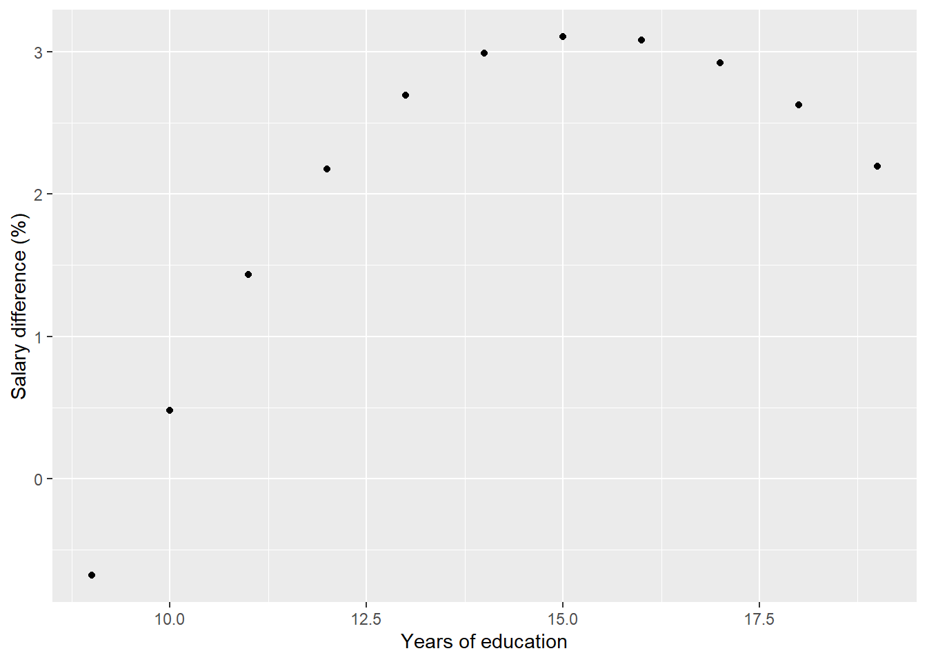
Figure 5: Model fit, SSYK 214, The derivative for education
Comparison between the categorical and the continuous predictor. Column withinconf states if the estimate from the numerical model is within the 95 % confidence interval from the Tukey’s honest significant difference table. All estimates from the model with the continuous predictor are within the 95 % confidence intervals from the Tukey HSD table.
tukeytable <- tukeytable %>%
  rowwise() %>%
  mutate(comp_from = unlist(strsplit(comparison, ")-"))[1]) %>%
  rowwise() %>%
  mutate(comp_to = unlist(strsplit(comparison, ")-"))[2]) %>%             mutate(comp_from = paste (comp_from, ")", sep="")) %>%
  left_join(numedulevel, by = c("comp_from" = "level.of.education")) %>%
  left_join(numedulevel, by = c("comp_to" = "level.of.education")) %>%    mutate(numestimate = predict(contspline, eduyears.x) -           predict(contspline, eduyears.y)) %>%
  mutate(withinconf = numestimate > conf.low && numestimate < conf.high) %>%
  mutate(percdiffcont = (1 / exp(predict(contspline, eduyears.x) - predict(contspline, eduyears.y)) - 1) * 100)
## Warning: Column `comp_from`/`level.of.education` joining character vector and
## factor, coercing into character vector## Warning: Column `comp_to`/`level.of.education` joining character vector and
## factor, coercing into character vectortukeytable %>%
select(term, comparison, estimate, adj.p.value, numestimate, withinconf, percdiff, percdiffcont) %>%
filter(adj.p.value < 0.05) %>%
arrange(estimate) %>%
knitr::kable(
booktabs = TRUE,
caption = 'Comparison between categorical and continous predictor')| term | comparison | estimate | adj.p.value | numestimate | withinconf | percdiff | percdiffcont |
|---|---|---|---|---|---|---|---|
| edulevel | primary and secondary education 9-10 years (ISCED97 2)-post-graduate education (ISCED97 6) | -0.2160450 | 0.0000000 | -0.2212179 | TRUE | 24.115819 | 24.7595300 |
| edulevel | upper secondary education, 2 years or less (ISCED97 3C)-post-graduate education (ISCED97 6) | -0.2155065 | 0.0000000 | -0.2123268 | TRUE | 24.049001 | 23.6551904 |
| edulevel | upper secondary education 3 years (ISCED97 3A)-post-graduate education (ISCED97 6) | -0.1898866 | 0.0000000 | -0.1942616 | TRUE | 20.911247 | 21.4413939 |
| edulevel | post-secondary education, less than 3 years (ISCED97 4+5B)-post-graduate education (ISCED97 6) | -0.1446573 | 0.0000001 | -0.1418336 | TRUE | 15.564352 | 15.2384840 |
| edulevel | post-secondary education 3 years or more (ISCED97 5A)-post-graduate education (ISCED97 6) | -0.1104356 | 0.0000443 | -0.1117048 | TRUE | 11.676444 | 11.8182726 |
| edulevel | primary and secondary education 9-10 years (ISCED97 2)-post-secondary education 3 years or more (ISCED97 5A) | -0.1056094 | 0.0001649 | -0.1095131 | TRUE | 11.138763 | 11.5734729 |
| edulevel | upper secondary education, 2 years or less (ISCED97 3C)-post-secondary education 3 years or more (ISCED97 5A) | -0.1050709 | 0.0001119 | -0.1006220 | TRUE | 11.078932 | 10.5858529 |
| edulevel | primary and secondary education 9-10 years (ISCED97 2)-no information about level of educational attainment | -0.1045888 | 0.0001950 | 0.0000000 | FALSE | 11.025400 | 0.0000000 |
| edulevel | upper secondary education, 2 years or less (ISCED97 3C)-no information about level of educational attainment | -0.1040503 | 0.0001331 | 0.0088912 | FALSE | 10.965630 | -0.8851746 |
| sex | women-men | -0.0803151 | 0.0000000 | 0.0000000 | FALSE | 8.362851 | 0.0000000 |
| edulevel | upper secondary education 3 years (ISCED97 3A)-post-secondary education 3 years or more (ISCED97 5A) | -0.0794510 | 0.0066749 | -0.0825568 | TRUE | 8.269249 | 8.6060365 |
| edulevel | upper secondary education 3 years (ISCED97 3A)-no information about level of educational attainment | -0.0784305 | 0.0077374 | 0.0269563 | FALSE | 8.158814 | -2.6596254 |
| edulevel | primary and secondary education 9-10 years (ISCED97 2)-post-secondary education, less than 3 years (ISCED97 4+5B) | -0.0713876 | 0.0264560 | -0.0793844 | TRUE | 7.399745 | 8.2620369 |
| edulevel | upper secondary education, 2 years or less (ISCED97 3C)-post-secondary education, less than 3 years (ISCED97 4+5B) | -0.0708491 | 0.0221087 | -0.0704932 | TRUE | 7.341926 | 7.3037289 |
| edulevel | post-graduate education (ISCED97 6)-no information about level of educational attainment | 0.1114561 | 0.0000370 | 0.2212179 | FALSE | -10.546938 | -19.8458026 |
Now. let´s perform some diagnostics on the models. First, a look at the residuals for the model shows no apparent problem. We can see that the outlier at row 55 has disappeared in the plots for the continuous model.
Three out of four outliers when using categorical predictors were from the factor “no information about level of educational attainment”.
For the continuous predictors there are two outliers in the factor “upper secondary education, 2 years or less (ISCED97 3C)” and two outliers in the factor “upper secondary education 3 years (ISCED97 3A)” indicating that the model could be improved.
tb[20,]$edulevel## [1] "no information about level of educational attainment"tb[41,]$edulevel## [1] "no information about level of educational attainment"tb[55,]$edulevel## [1] "no information about level of educational attainment"tb[57,]$edulevel## [1] "upper secondary education, 2 years or less (ISCED97 3C)"tbnum[12,]$edulevel## [1] "upper secondary education, 2 years or less (ISCED97 3C)"tbnum[18,]$edulevel## [1] "upper secondary education, 2 years or less (ISCED97 3C)"tbnum[25,]$edulevel## [1] "upper secondary education 3 years (ISCED97 3A)"tbnum[29,]$edulevel## [1] "upper secondary education 3 years (ISCED97 3A)"plot(model, which = 1)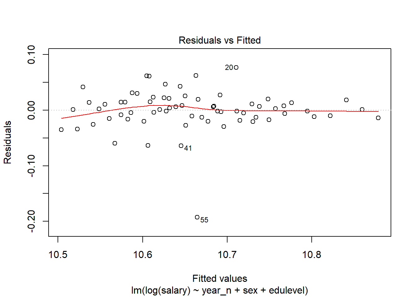
Figure 6: Residuals vs Fitted of model fit
plot(modelcont, which = 1)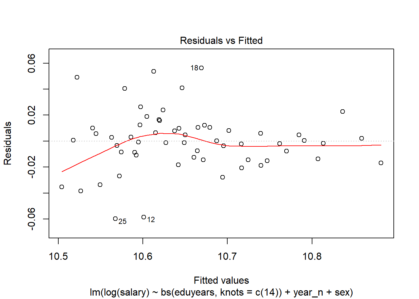
Figure 7: Residuals vs Fitted of model fit
The Normal Q-Q shows some possible outliers.
plot(model, which = 2)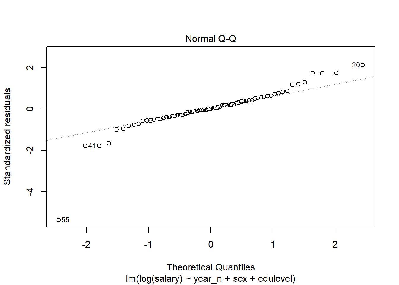
Figure 8: Normal Q-Q
plot(modelcont, which = 2)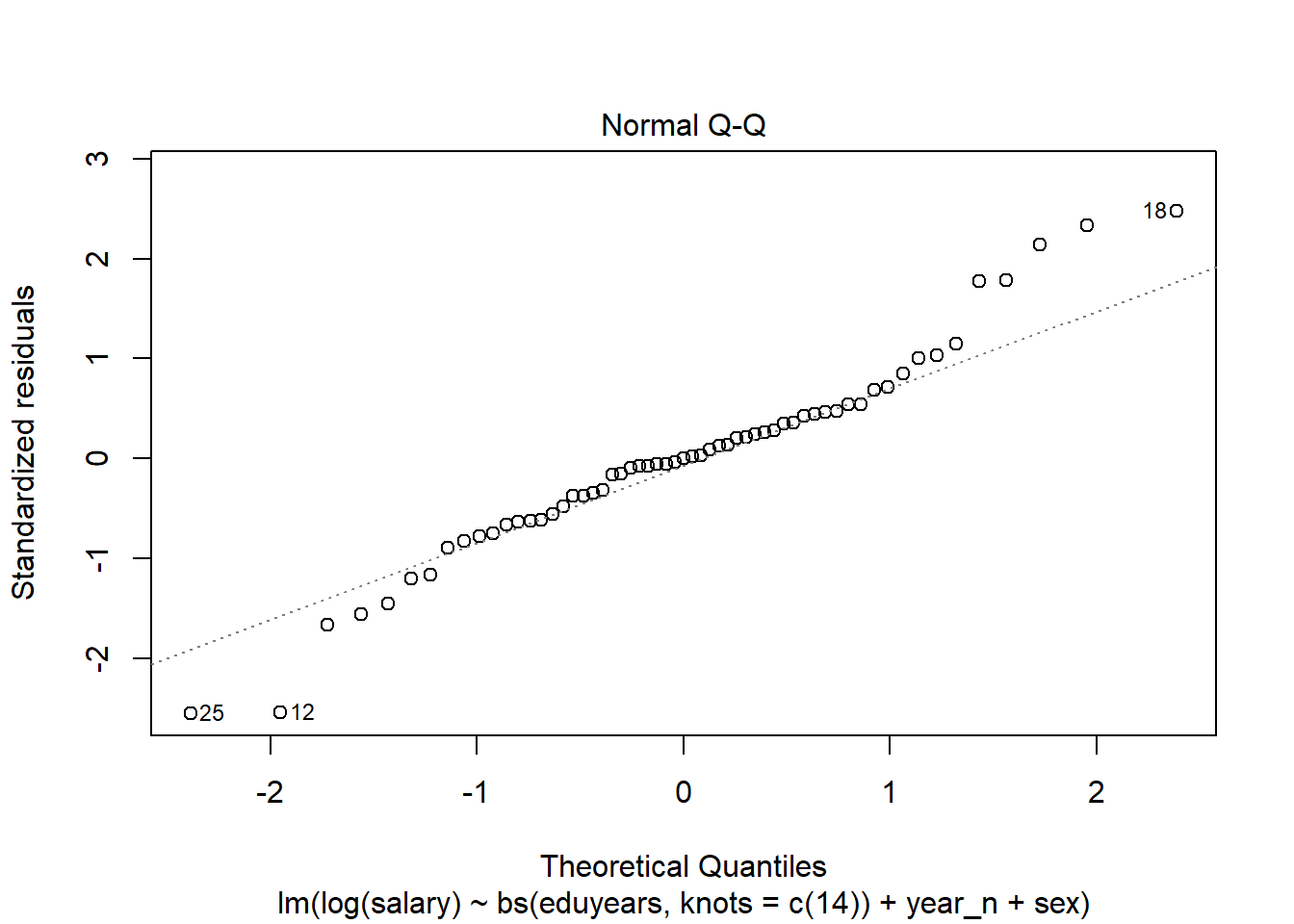
Figure 9: Normal Q-Q
Again, the Standardised residuals show some possible outliers.
plot(model, which = 3)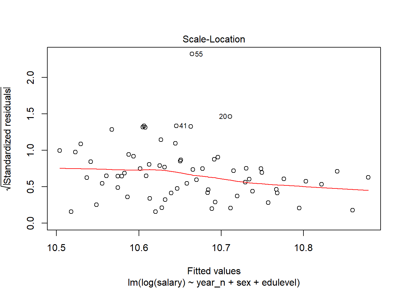
Figure 10: Scale-Location
plot(modelcont, which = 3)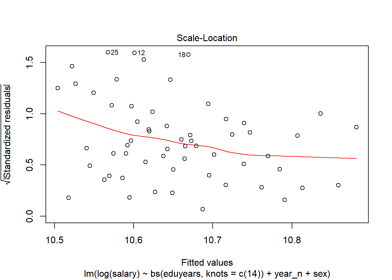
Figure 11: Scale-Location
The outliers are also found in the Leverage plot.
plot(model, which = 5)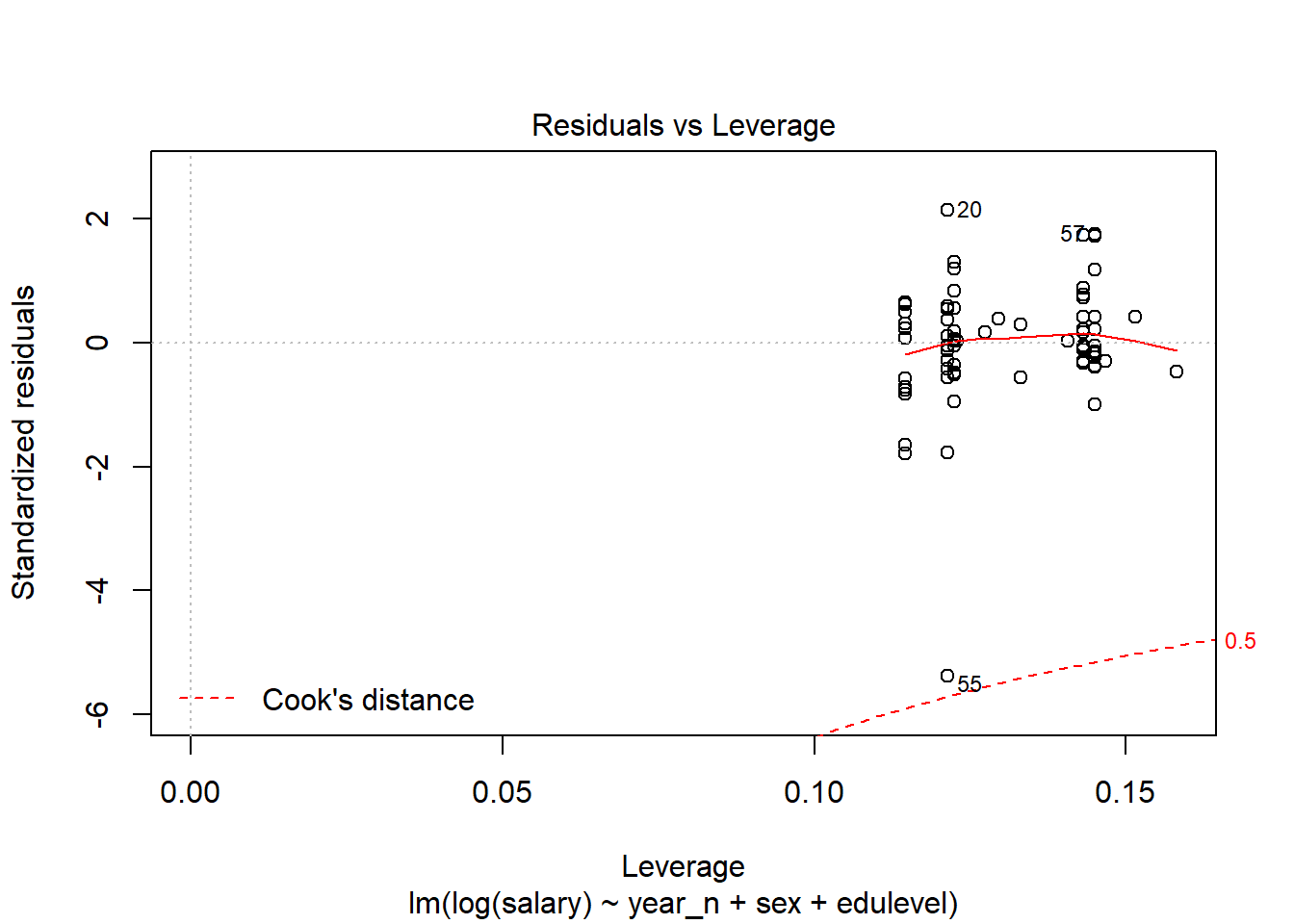
Figure 12: Residuals vs Leverage
plot(modelcont, which = 5)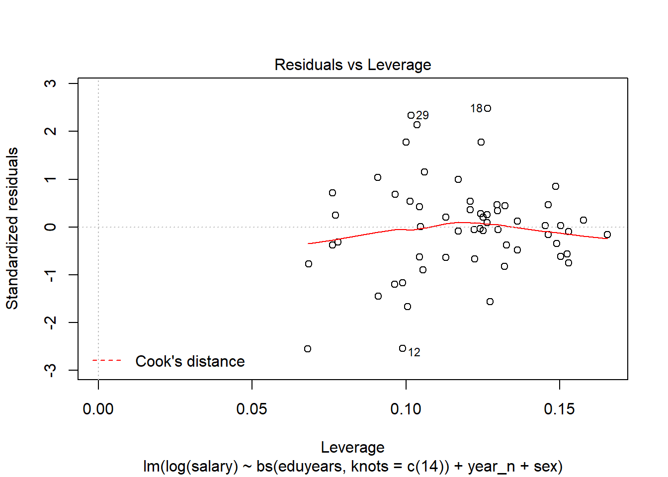
Figure 13: Residuals vs Leverage