In my last post, I found that education has a significant impact on the salary of engineers. Is the significance of education on wages unique to engineers or are there similar correlations in other occupational groups?
I will use the same model in principal as in my previous post to calculate the significance of education. I will not use sex as an explanatory variable since there are occupational groups that do not have enough data for both genders. Searching through the different occupational groups I will fit education with a polynomial of degree one. I am interested in occupational groups where a longer education also results in higher salaries. Because of that, I will use the numerical approximation from my last post instead of using the categorical predictor. A polynomial of higher degree than one would result in a better fit but the problem with oscillation and overfitting made me settle for degree one. A straight line as a function also has the advantage that the average increase in salary for each education year is directly given from the model.
There are still occupational groups with too little data for regression analysis. More than 30 posts are necessary to fit both education and year.
The F-value from the Anova table is used as the single value to discriminate how much education and salary correlates. For exploratory analysis, the Anova value seems good enough.
In the figure below I will also use the estimate for education to see how much the salaries are raised by education for the different occupational groups holding year as constant.
library (tidyverse)## -- Attaching packages ------------------------------------------- tidyverse 1.2.1 --## v ggplot2 3.2.0 v purrr 0.3.2
## v tibble 2.1.3 v dplyr 0.8.3
## v tidyr 0.8.3 v stringr 1.4.0
## v readr 1.3.1 v forcats 0.4.0## -- Conflicts ---------------------------------------------- tidyverse_conflicts() --
## x dplyr::filter() masks stats::filter()
## x dplyr::lag() masks stats::lag()library (broom)
library (car)## Loading required package: carData##
## Attaching package: 'car'## The following object is masked from 'package:dplyr':
##
## recode## The following object is masked from 'package:purrr':
##
## somelibrary (splines)
#install_github("ZheyuanLi/SplinesUtils")
library (SplinesUtils)
readfile <- function (file1){read_csv (file1, col_types = cols(), locale = readr::locale (encoding = "latin1"), na = c("..", "NA")) %>%
gather (starts_with("19"), starts_with("20"), key = "year", value = salary) %>%
drop_na() %>%
mutate (year_n = parse_number (year))
}The data table is downloaded from Statistics Sweden. It is saved as a comma-delimited file without heading, 000000CY.csv, http://www.statistikdatabasen.scb.se/pxweb/en/ssd/.
The table: Average basic salary, monthly salary and women´s salary as a percentage of men´s salary by sector, occupational group (SSYK 2012), sex and educational level (SUN). Year 2014 - 2018 Monthly salary All sectors
tb <- readfile("000000CY.csv")

numedulevel <- read.csv("edulevel.csv")

numedulevel %>%
  knitr::kable(
  booktabs = TRUE,
caption = 'Initial approach, length of education') | level.of.education | eduyears |
|---|---|
| primary and secondary education 9-10 years (ISCED97 2) | 9 |
| upper secondary education, 2 years or less (ISCED97 3C) | 11 |
| upper secondary education 3 years (ISCED97 3A) | 12 |
| post-secondary education, less than 3 years (ISCED97 4+5B) | 14 |
| post-secondary education 3 years or more (ISCED97 5A) | 15 |
| post-graduate education (ISCED97 6) | 19 |
| no information about level of educational attainment | NA |
tbnum <- tb %>%
  right_join(numedulevel, by = c("level of education" = "level.of.education")) %>%
  filter(!is.na(eduyears))
## Warning: Column `level of education`/`level.of.education` joining character
## vector and factor, coercing into character vectorsummary_table = vector()
anova_table = vector()
for (i in unique(tbnum$`occuptional (SSYK 2012)`)){
temp <- filter(tbnum, `occuptional (SSYK 2012)` == i)
if (dim(temp)[1] > 30){
model <- lm (log(salary) ~ year_n + eduyears, data = temp)
summary_table <- rbind (summary_table, mutate (tidy (summary (model)), ssyk = i))
anova_table <- rbind (anova_table, mutate (tidy (Anova (model, type = 2)), ssyk = i))
}
}
merge(summary_table, anova_table, by = "ssyk", all = TRUE) %>%
filter (term.y == "eduyears") %>%
filter (term.x == "eduyears") %>%
mutate (estimate = (exp(estimate) - 1) * 100) %>%
ggplot () +
geom_point (mapping = aes(x = estimate, y = statistic.y)) +
labs(
x = "Increase in salaries (% / year of education)",
y = "F-value for education"
) 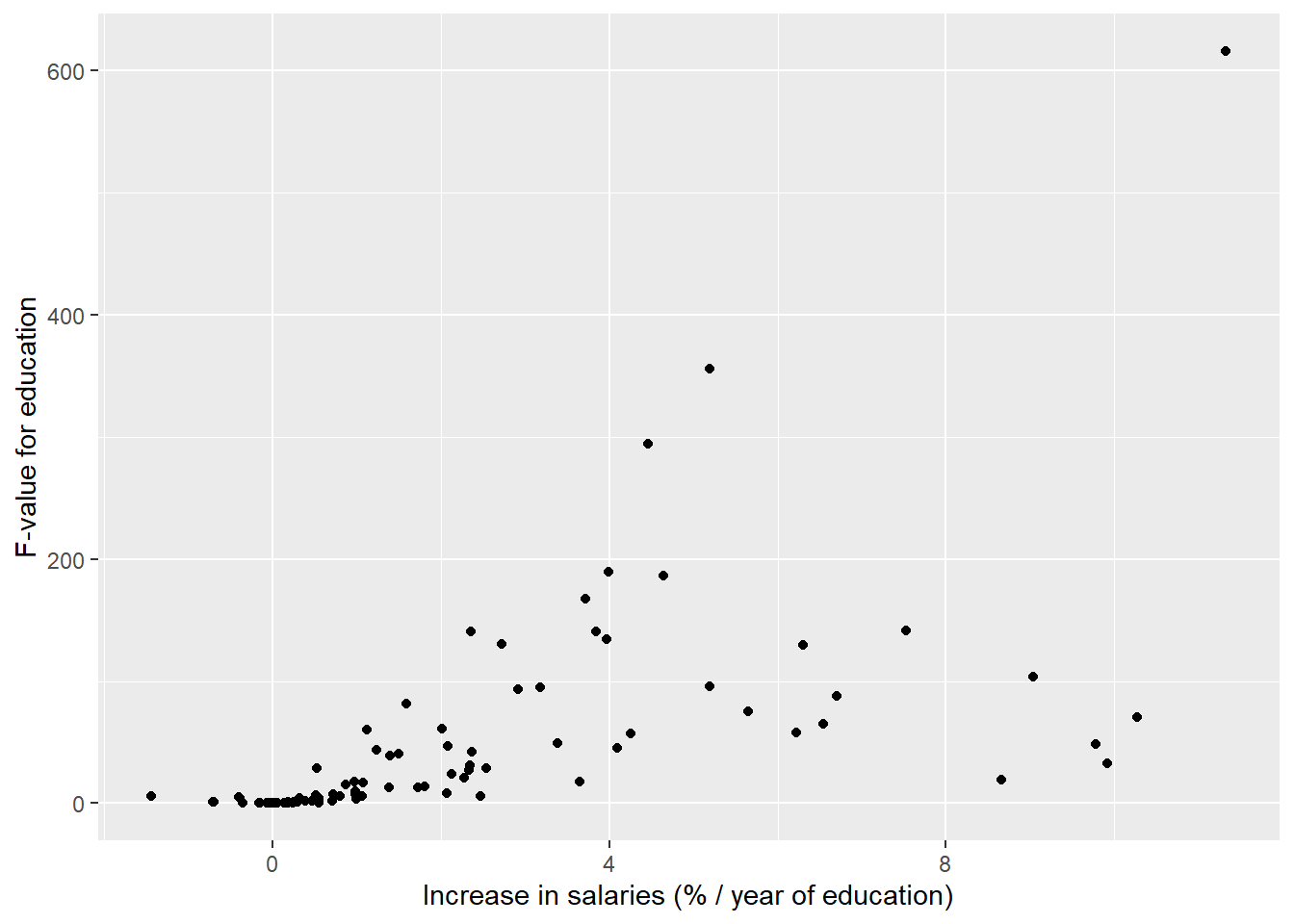
Figure 1: The significance of education on the salary in Sweden, a comparison between different occupational groups, Year 2014 - 2018
The table with all occupational groups sorted by Increase in salary in descending order.
merge(summary_table, anova_table, by = "ssyk", all = TRUE) %>%
  filter (term.y == "eduyears") %>%
  filter (term.x == "eduyears") %>%
  select (ssyk, estimate, statistic.y) %>%
  mutate (estimate = (exp(estimate) - 1) * 100) %>%
  rename (`F-value for education` = statistic.y) %>%
  rename (`Increase in salary` = estimate) %>%
  arrange (desc (`Increase in salary`)) %>%
  knitr::kable(
    booktabs = TRUE,
caption = 'Correlation for F-value (education) and the increase in salaries for each year of education')| ssyk | Increase in salary | F-value for education |
|---|---|---|
| 151 Health care managers | 11.3222562 | 615.8861538 |
| 221 Medical doctors | 10.2650113 | 70.5835974 |
| 121 Finance managers | 9.9172689 | 32.7350353 |
| 261 Legal professionals | 9.7834120 | 48.1004817 |
| 122 Human resource managers | 9.0394770 | 103.8231602 |
| 161 Financial and insurance managers | 8.6603822 | 19.2527280 |
| 231 University and higher education teachers | 7.5276294 | 141.4796497 |
| 132 Supply, logistics and transport managers | 6.6969576 | 87.6384397 |
| 137 Production managers in manufacturing | 6.5378753 | 65.2842719 |
| 123 Administration and planning managers | 6.2977859 | 129.4982036 |
| 136 Production managers in construction and mining | 6.2192630 | 57.8361291 |
| 129 Administration and service managers not elsewhere classified | 5.6522431 | 74.9238199 |
| 131 Information and communications technology service managers | 5.1937185 | 95.3092758 |
| 159 Other social services managers | 5.1920288 | 355.8557670 |
| 134 Architectural and engineering managers | 4.6458339 | 186.5137309 |
| 262 Museum curators and librarians and related professionals | 4.4638502 | 294.6004878 |
| 332 Insurance advisers, sales and purchasing agents | 4.2505985 | 57.1999444 |
| 179 Other services managers not elsewhere classified | 4.0931013 | 44.9824826 |
| 235 Teaching professionals not elsewhere classified | 3.9957394 | 189.3385229 |
| 311 Physical and engineering science technicians | 3.9729301 | 134.6441603 |
| 234 Primary- and pre-school teachers | 3.8498852 | 140.3499938 |
| 233 Secondary education teachers | 3.7146273 | 167.3564935 |
| 125 Sales and marketing managers | 3.6489071 | 17.5675213 |
| 241 Accountants, financial analysts and fund managers | 3.3820710 | 49.5445027 |
| 242 Organisation analysts, policy administrators and human resource specialists | 3.1833018 | 94.6038730 |
| 213 Biologists, pharmacologists and specialists in agriculture and forestry | 2.9242020 | 93.6360138 |
| 321 Medical and pharmaceutical technicians | 2.7274994 | 130.1793959 |
| 133 Research and development managers | 2.5377568 | 28.8355719 |
| 173 Retail and wholesale trade managers | 2.4736675 | 5.9078862 |
| 335 Tax and related government associate professionals | 2.3658837 | 41.8703194 |
| 214 Engineering professionals | 2.3546977 | 140.9367261 |
| 243 Marketing and public relations professionals | 2.3458276 | 31.1353096 |
| 232 Vocational education teachers | 2.3303514 | 27.2589020 |
| 334 Administrative and specialized secretaries | 2.2765069 | 20.8078772 |
| 342 Athletes, fitness instructors and recreational workers | 2.1279403 | 24.0465329 |
| 266 Social work and counselling professionals | 2.0818202 | 46.6894573 |
| 331 Financial and accounting associate professionals | 2.0726916 | 8.1402279 |
| 411 Office assistants and other secretaries | 2.0115047 | 60.8893100 |
| 523 Cashiers and related clerks | 1.8137124 | 13.9599411 |
| 524 Event seller and telemarketers | 1.7261688 | 13.0208742 |
| 251 ICT architects, systems analysts and test managers | 1.5958484 | 81.4664709 |
| 819 Process control technicians | 1.4963794 | 40.1366829 |
| 962 Newspaper distributors, janitors and other service workers | 1.3940863 | 38.9982657 |
| 812 Metal processing and finishing plant operators | 1.3878292 | 12.9570916 |
| 432 Stores and transport clerks | 1.2376483 | 43.6773646 |
| 341 Social work and religious associate professionals | 1.1195539 | 60.5012820 |
| 531 Child care workers and teachers aides | 1.0815506 | 16.6066709 |
| 264 Authors, journalists and linguists | 1.0636388 | 5.4839869 |
| 333 Business services agents | 1.0019699 | 3.5614940 |
| 522 Shop staff | 0.9835325 | 9.4858527 |
| 351 ICT operations and user support technicians | 0.9821077 | 7.4180769 |
| 441 Library and filing clerks | 0.9770931 | 17.5562894 |
| 941 Fast-food workers, food preparation assistants | 0.8675015 | 15.3917476 |
| 611 Market gardeners and crop growers | 0.8014313 | 6.0302572 |
| 817 Wood processing and papermaking plant operators | 0.7291227 | 7.4060017 |
| 217 Designers | 0.7088900 | 1.8475401 |
| 831 Train operators and related workers | 0.5548934 | 3.3520151 |
| 932 Manufacturing labourers | 0.5533498 | 4.2142587 |
| 343 Photographers, interior decorators and entertainers | 0.5498463 | 0.6786136 |
| 513 Waiters and bartenders | 0.5489340 | 2.0997794 |
| 312 Construction and manufacturing supervisors | 0.5475032 | 1.3980603 |
| 534 Attendants, personal assistants and related workers | 0.5264678 | 28.8067668 |
| 515 Building caretakers and related workers | 0.5221112 | 6.8499176 |
| 815 Machine operators, textile, fur and leather products | 0.4691193 | 2.1375421 |
| 422 Client information clerks | 0.3886323 | 1.7115048 |
| 533 Health care assistants | 0.3239149 | 4.1630503 |
| 818 Other stationary plant and machine operators | 0.2957261 | 1.0364217 |
| 512 Cooks and cold-buffet managers | 0.2548134 | 0.9265992 |
| 711 Carpenters, bricklayers and construction workers | 0.2417011 | 0.1572365 |
| 218 Specialists within environmental and health protection | 0.2397413 | 0.4222318 |
| 961 Recycling collectors | 0.1921605 | 0.8568597 |
| 541 Other surveillance and security workers | 0.1812197 | 0.4153472 |
| 511 Cabin crew, guides and related workers | 0.1658380 | 0.2150479 |
| 723 Machinery mechanics and fitters | 0.1410149 | 0.2170183 |
| 821 Assemblers | 0.0644892 | 0.0858323 |
| 813 Machine operators, chemical and pharmaceutical products | 0.0326476 | 0.0217158 |
| 833 Heavy truck and bus drivers | 0.0309875 | 0.0482259 |
| 816 Machine operators, food and related products | 0.0069780 | 0.0017000 |
| 532 Personal care workers in health services | -0.0383003 | 0.1216850 |
| 352 Broadcasting and audio-visual technicians | -0.0705932 | 0.0171995 |
| 814 Machine operators, rubber, plastic and paper products | -0.1428982 | 0.2504506 |
| 722 Blacksmiths, toolmakers and related trades workers | -0.1569686 | 0.4841203 |
| 732 Printing trades workers | -0.3543764 | 0.5477171 |
| 911 Cleaners and helpers | -0.3859718 | 4.5299051 |
| 834 Mobile plant operators | -0.3979938 | 5.1952942 |
| 216 Architects and surveyors | -0.6970606 | 1.2794827 |
| 516 Other service related workers | -0.7106422 | 1.0123452 |
| 265 Creative and performing artists | -1.4326841 | 6.0250927 |
Let’s check what we have found.
temp <- tbnum %>%
  filter(`occuptional  (SSYK 2012)` == "151 Health care managers")

temp %>%
  ggplot () +
    geom_point (mapping = aes(x = year_n,y = salary, colour = eduyears)) +
    facet_grid(. ~ sex) +
    labs(
      x = "Year",
      y = "Salary (SEK/month)"
) 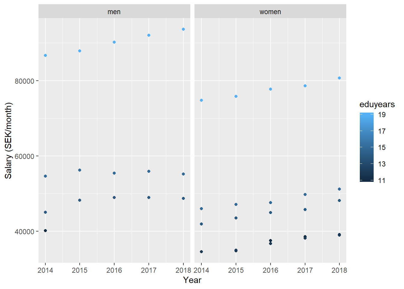
Figure 2: Highest increase in salary, 151 Health care managers
modelcont <- lm (log(salary) ~ year_n + bs(eduyears, degree = 1), data = temp)

contspline <- RegBsplineAsPiecePoly(modelcont, "bs(eduyears, degree = 1)")

tibble(eduyears = seq(11, 19, by=0.1)) %>%
  ggplot () +
    geom_point (mapping = aes(x = eduyears,y = predict(contspline, eduyears))) +
  labs(
    x = "Years of education",
    y = "Salary"
  )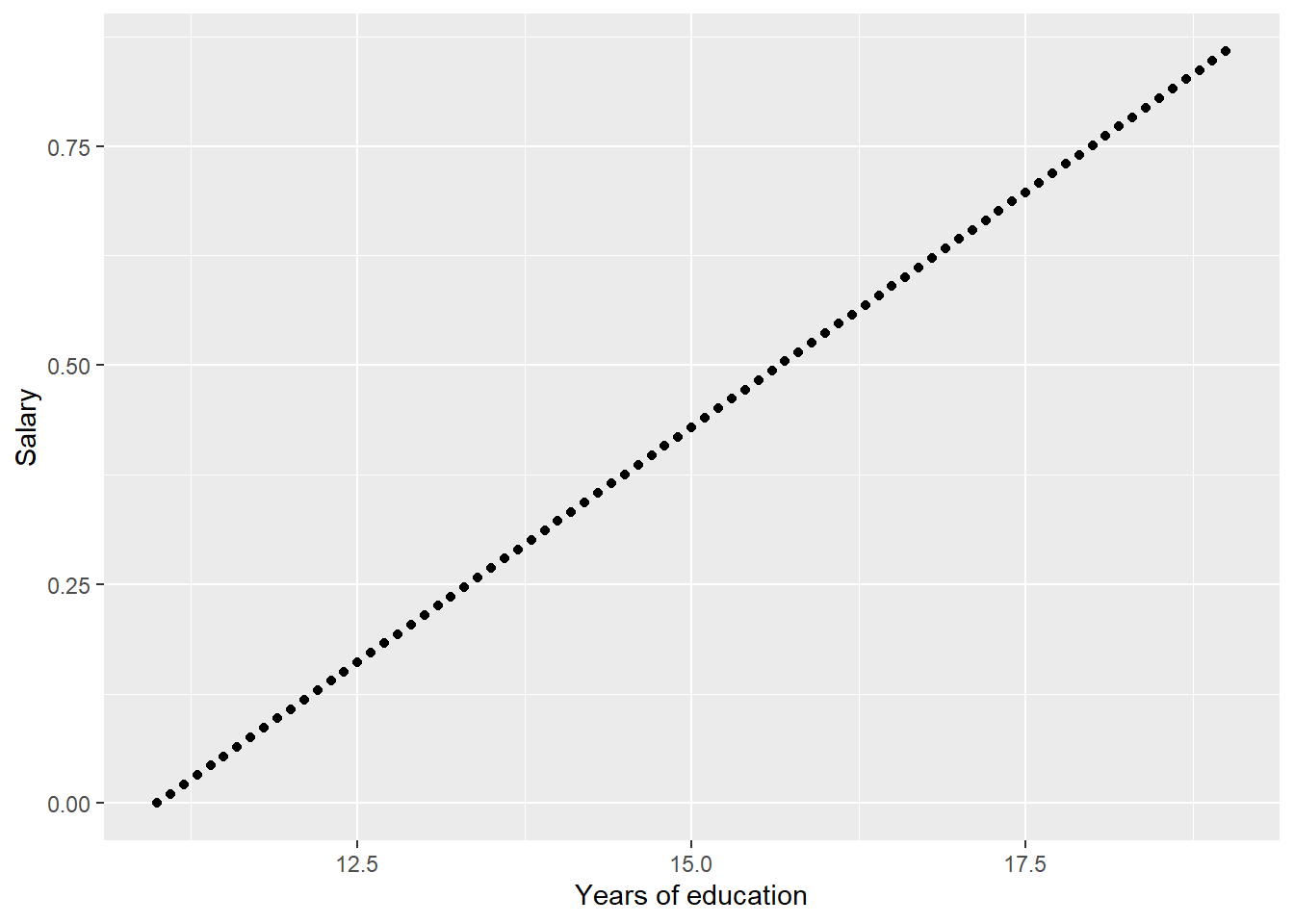
Figure 3: Model fit, Health care managers, Correlation between education and salary
tibble(eduyears = seq(11, 19, by=0.1)) %>%
  ggplot () +
    geom_point (mapping = aes(x = eduyears,y = (exp(predict(contspline, eduyears, deriv = 1)) - 1) * 100)) +
  labs(
    x = "Years of education",
    y = "Salary difference (%)"
  )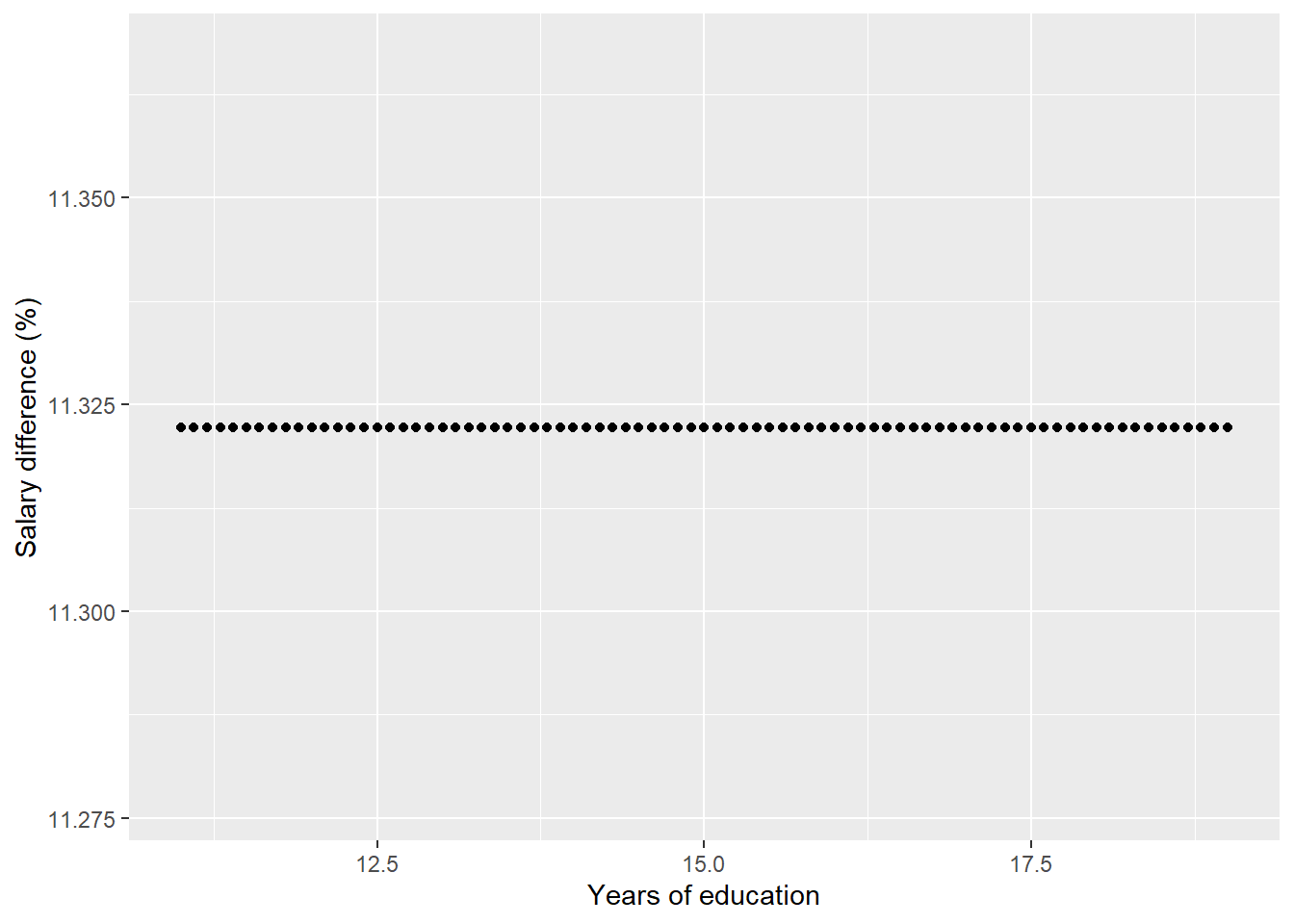
Figure 4: Model fit, Health care managers, The derivative for educaton
temp <- tbnum %>%
  filter(`occuptional  (SSYK 2012)` == "265 Creative and performing artists")

temp %>%
  ggplot () +
    geom_point (mapping = aes(x = year_n,y = salary, colour = eduyears)) +
    facet_grid(. ~ sex) +
    labs(
      x = "Year",
      y = "Salary (SEK/month)"
) 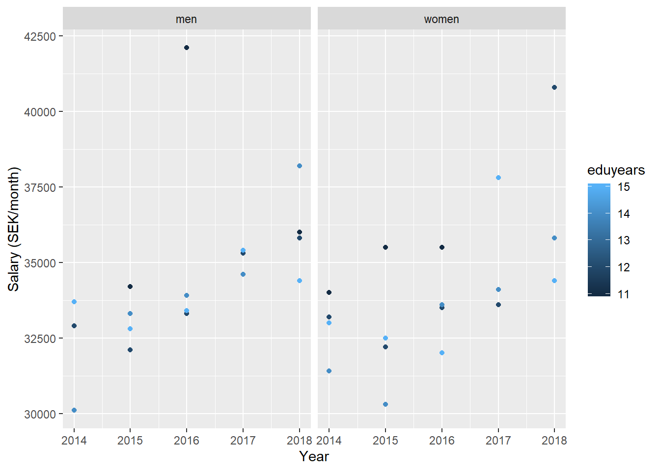
Figure 5: Lowest increase in salary, 265 Creative and performing artists
modelcont <- lm (log(salary) ~ year_n + bs(eduyears, degree = 1), data = temp)

contspline <- RegBsplineAsPiecePoly(modelcont, "bs(eduyears, degree = 1)")

tibble(eduyears = seq(11, 15, by=0.1)) %>%
  ggplot () +
    geom_point (mapping = aes(x = eduyears,y = predict(contspline, eduyears))) +
  labs(
    x = "Years of education",
    y = "Salary"
  )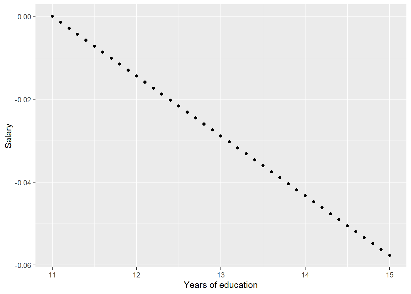
Figure 6: Model fit, Creative and performing artists, Correlation between education and salary
tibble(eduyears = seq(11, 15, by=0.1)) %>%
  ggplot () +
    geom_point (mapping = aes(x = eduyears,y = (exp(predict(contspline, eduyears, deriv = 1)) - 1) * 100)) +
  labs(
    x = "Years of education",
    y = "Salary difference (%)"
  )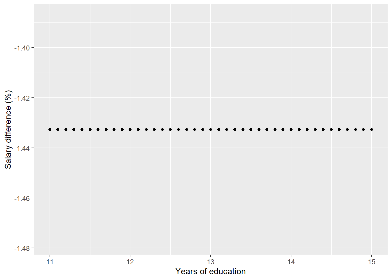
Figure 7: Model fit, Creative and performing artists, The derivative for education