In my previous posts, I have shown that there exists a correlation between salaries and experience as well as between salaries and education within many occupational groups. Within the data I used from Statistics Sweden there was also information about gender. Some of the models and graphs also showed that there is a difference in salaries between the different genders.
In this post, I will examine the interaction between the predictors. Apart from gender the interaction between year also needs to be investigated.
It would have been very interesting to examine the interaction between experience and education. However, this information is not available at Statistics Sweden, at least not for free.
First, define libraries and functions.
library (tidyverse) ## -- Attaching packages --------------------------------------- tidyverse 1.2.1 --## v ggplot2 3.2.0 v purrr 0.3.2
## v tibble 2.1.3 v dplyr 0.8.3
## v tidyr 1.0.0 v stringr 1.4.0
## v readr 1.3.1 v forcats 0.4.0## -- Conflicts ------------------------------------------ tidyverse_conflicts() --
## x dplyr::filter() masks stats::filter()
## x dplyr::lag() masks stats::lag()library (broom)
library (car)## Loading required package: carData##
## Attaching package: 'car'## The following object is masked from 'package:dplyr':
##
## recode## The following object is masked from 'package:purrr':
##
## somelibrary (splines)
#install_github("ZheyuanLi/SplinesUtils")
library(SplinesUtils)
library(sjPlot)
readfile <- function (file1){
read_csv (file1, col_types = cols(), locale = readr::locale (encoding = "latin1"), na = c("..", "NA")) %>%
gather (starts_with("19"), starts_with("20"), key = "year", value = salary) %>%
drop_na() %>%
mutate (year_n = parse_number (year))
}The data table is downloaded from Statistics Sweden. It is saved as a comma-delimited file without heading, 00000031.csv, http://www.statistikdatabasen.scb.se/pxweb/en/ssd/.
Average monthly pay (total pay), non-manual workers private sector (SLP), SEK by occupational group (SSYK), age, sex and year. Year 2014 - 2018
There are no women in the age group 65-66 years which explains the uncertainty for this group.
We are interested to see if the interaction terms between gender, age and year are important factors in salaries. As a null hypothesis, we assume that the interaction terms between gender, age and year is not related to the salary and examine if we can reject this hypothesis with the data from Statistics Sweden.
tb <- readfile("00000031.csv") %>%
  rowwise() %>%
  mutate(age_l = unlist(lapply(strsplit(substr(age, 1, 5), "-"), strtoi))[1]) %>%
  rowwise() %>%
  mutate(age_h = unlist(lapply(strsplit(substr(age, 1, 5), "-"), strtoi))[2]) %>%
  mutate(age_n = (age_l + age_h) / 2)

tb %>%
  ggplot () +
    geom_point (mapping = aes(x = year_n,y = salary, colour = age, shape = sex)) +
  labs(
    x = "Year",
    y = "Salary (SEK/month)"
  )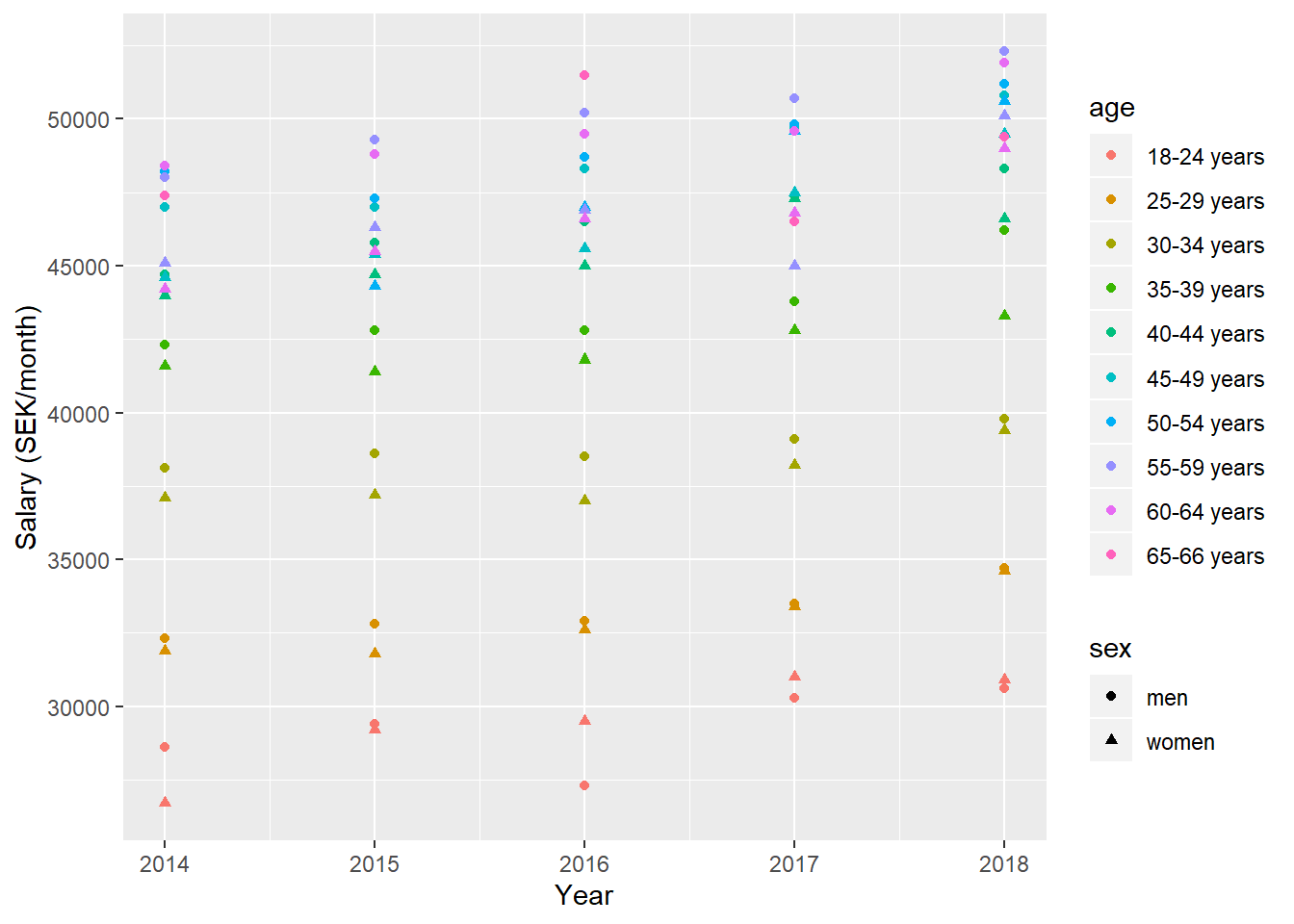
Figure 1: SSYK 214, Architects, engineers and related professionals, Year 2014 - 2018
model <- lm (log(salary) ~ year_n + sex + age, data = tb)

summary(model) %>%
  tidy() %>%
  knitr::kable(
  booktabs = TRUE,
caption = 'Summary from linear model fit')| term | estimate | std.error | statistic | p.value |
|---|---|---|---|---|
| (Intercept) | -28.1818327 | 3.5502758 | -7.937928 | 0 |
| year_n | 0.0190896 | 0.0017610 | 10.839936 | 0 |
| sexwomen | -0.0338702 | 0.0051006 | -6.640420 | 0 |
| age25-29 years | 0.1194646 | 0.0108200 | 11.041048 | 0 |
| age30-34 years | 0.2670157 | 0.0108200 | 24.677885 | 0 |
| age35-39 years | 0.3798043 | 0.0108200 | 35.101929 | 0 |
| age40-44 years | 0.4507298 | 0.0108200 | 41.656942 | 0 |
| age45-49 years | 0.4826082 | 0.0108200 | 44.603178 | 0 |
| age50-54 years | 0.4957858 | 0.0108200 | 45.821064 | 0 |
| age55-59 years | 0.4999386 | 0.0108200 | 46.204870 | 0 |
| age60-64 years | 0.4926852 | 0.0108200 | 45.534501 | 0 |
| age65-66 years | 0.4850540 | 0.0145457 | 33.346995 | 0 |
summary(model)$adj.r.squared ## [1] 0.9817476Anova(model, type = 2)## Anova Table (Type II tests)
##
## Response: log(salary)
## Sum Sq Df F value Pr(>F)
## year_n 0.06878 1 117.504 < 2.2e-16 ***
## sex 0.02581 1 44.095 3.166e-09 ***
## age 2.81366 9 534.074 < 2.2e-16 ***
## Residuals 0.04800 82
## ---
## Signif. codes: 0 '***' 0.001 '**' 0.01 '*' 0.05 '.' 0.1 ' ' 1plot(model, which = 1)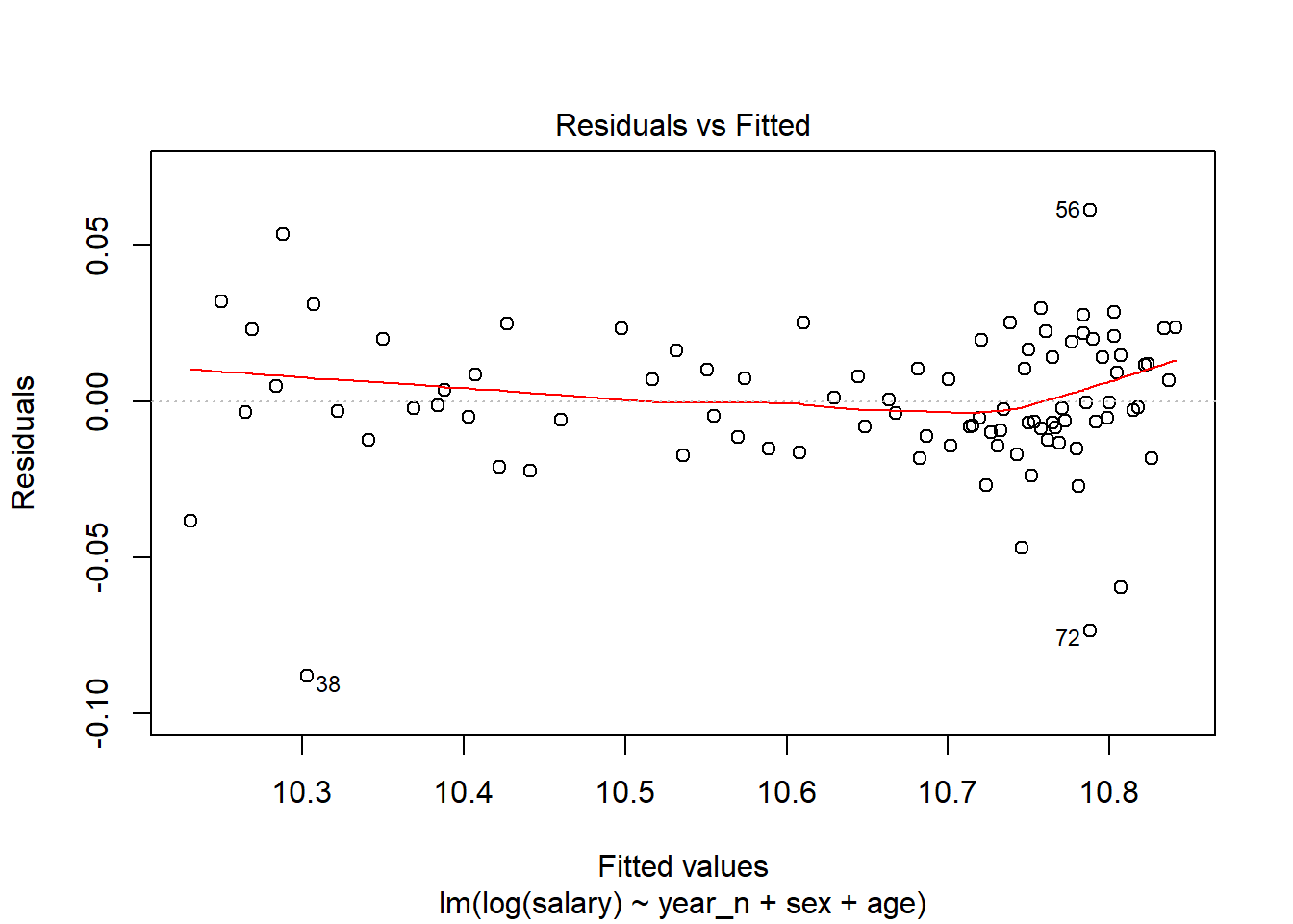
Figure 2: SSYK 214, Architects, engineers and related professionals, Year 2014 - 2018
tb[38,]## Source: local data frame [1 x 9]
## Groups: <by row>
##
## # A tibble: 1 x 9
## `occuptional (SSYK 2012~ age sex year salary year_n age_l age_h age_n
## <chr> <chr> <chr> <chr> <dbl> <dbl> <int> <int> <dbl>
## 1 214 Engineering professi~ 18-24 y~ men 2016 27300 2016 18 24 21tb[56,]## Source: local data frame [1 x 9]
## Groups: <by row>
##
## # A tibble: 1 x 9
## `occuptional (SSYK 2012~ age sex year salary year_n age_l age_h age_n
## <chr> <chr> <chr> <chr> <dbl> <dbl> <int> <int> <dbl>
## 1 214 Engineering professi~ 65-66 y~ men 2016 51500 2016 65 66 65.5tb[72,]## Source: local data frame [1 x 9]
## Groups: <by row>
##
## # A tibble: 1 x 9
## `occuptional (SSYK 2012~ age sex year salary year_n age_l age_h age_n
## <chr> <chr> <chr> <chr> <dbl> <dbl> <int> <int> <dbl>
## 1 214 Engineering professi~ 55-59 y~ women 2017 45000 2017 55 59 57I will examine models with both the categorical and continuous predictors to see if they can make the same predictions. The models with continuous predictors show approximately the same as the models with categorical predictors as you can see below.
We start by examining the interaction between year and age. We find that the only significant interaction between age and year is in the age group 65-66 years old.
model <- lm (log(salary) ~ sex + year_n * age, data = tb)

summary(model) %>%
  tidy() %>%
  knitr::kable(
  booktabs = TRUE,
caption = 'Summary from linear model fit')| term | estimate | std.error | statistic | p.value |
|---|---|---|---|---|
| (Intercept) | -41.8453794 | 10.9079056 | -3.8362433 | 0.0002631 |
| sexwomen | -0.0338702 | 0.0051012 | -6.6396284 | 0.0000000 |
| year_n | 0.0258672 | 0.0054107 | 4.7807733 | 0.0000088 |
| age25-29 years | 14.3621579 | 15.4261077 | 0.9310293 | 0.3549073 |
| age30-34 years | 27.5176359 | 15.4261077 | 1.7838353 | 0.0786064 |
| age35-39 years | 20.9934100 | 15.4261077 | 1.3609013 | 0.1777316 |
| age40-44 years | 16.2491631 | 15.4261077 | 1.0533547 | 0.2956526 |
| age45-49 years | 5.7537717 | 15.4261077 | 0.3729892 | 0.7102373 |
| age50-54 years | 0.6906147 | 15.4261077 | 0.0447692 | 0.9644135 |
| age55-59 years | 14.2039759 | 15.4261077 | 0.9207751 | 0.3602008 |
| age60-64 years | 13.3026500 | 15.4261077 | 0.8623465 | 0.3913210 |
| age65-66 years | 44.0644781 | 19.7739637 | 2.2284090 | 0.0289332 |
| year_n:age25-29 years | -0.0070648 | 0.0076518 | -0.9232852 | 0.3589003 |
| year_n:age30-34 years | -0.0135172 | 0.0076518 | -1.7665264 | 0.0814879 |
| year_n:age35-39 years | -0.0102250 | 0.0076518 | -1.3362808 | 0.1856080 |
| year_n:age40-44 years | -0.0078365 | 0.0076518 | -1.0241363 | 0.3091527 |
| year_n:age45-49 years | -0.0026147 | 0.0076518 | -0.3417041 | 0.7335553 |
| year_n:age50-54 years | -0.0000966 | 0.0076518 | -0.0126298 | 0.9899576 |
| year_n:age55-59 years | -0.0067976 | 0.0076518 | -0.8883667 | 0.3772614 |
| year_n:age60-64 years | -0.0063541 | 0.0076518 | -0.8304083 | 0.4090156 |
| year_n:age65-66 years | -0.0216149 | 0.0098077 | -2.2038822 | 0.0306865 |
summary(model)$adj.r.squared ## [1] 0.9817432Anova(model, type = 2)## Anova Table (Type II tests)
##
## Response: log(salary)
## Sum Sq Df F value Pr(>F)
## sex 0.02581 1 44.0847 4.817e-09 ***
## year_n 0.06878 1 117.4762 < 2.2e-16 ***
## age 2.81366 9 533.9464 < 2.2e-16 ***
## year_n:age 0.00526 9 0.9978 0.4497
## Residuals 0.04274 73
## ---
## Signif. codes: 0 '***' 0.001 '**' 0.01 '*' 0.05 '.' 0.1 ' ' 1plot_model(model, type = "pred", terms = c("year_n", "age"), colors = "Set3")## Model has log-transformed response. Back-transforming predictions to original response scale. Standard errors are still on the log-scale.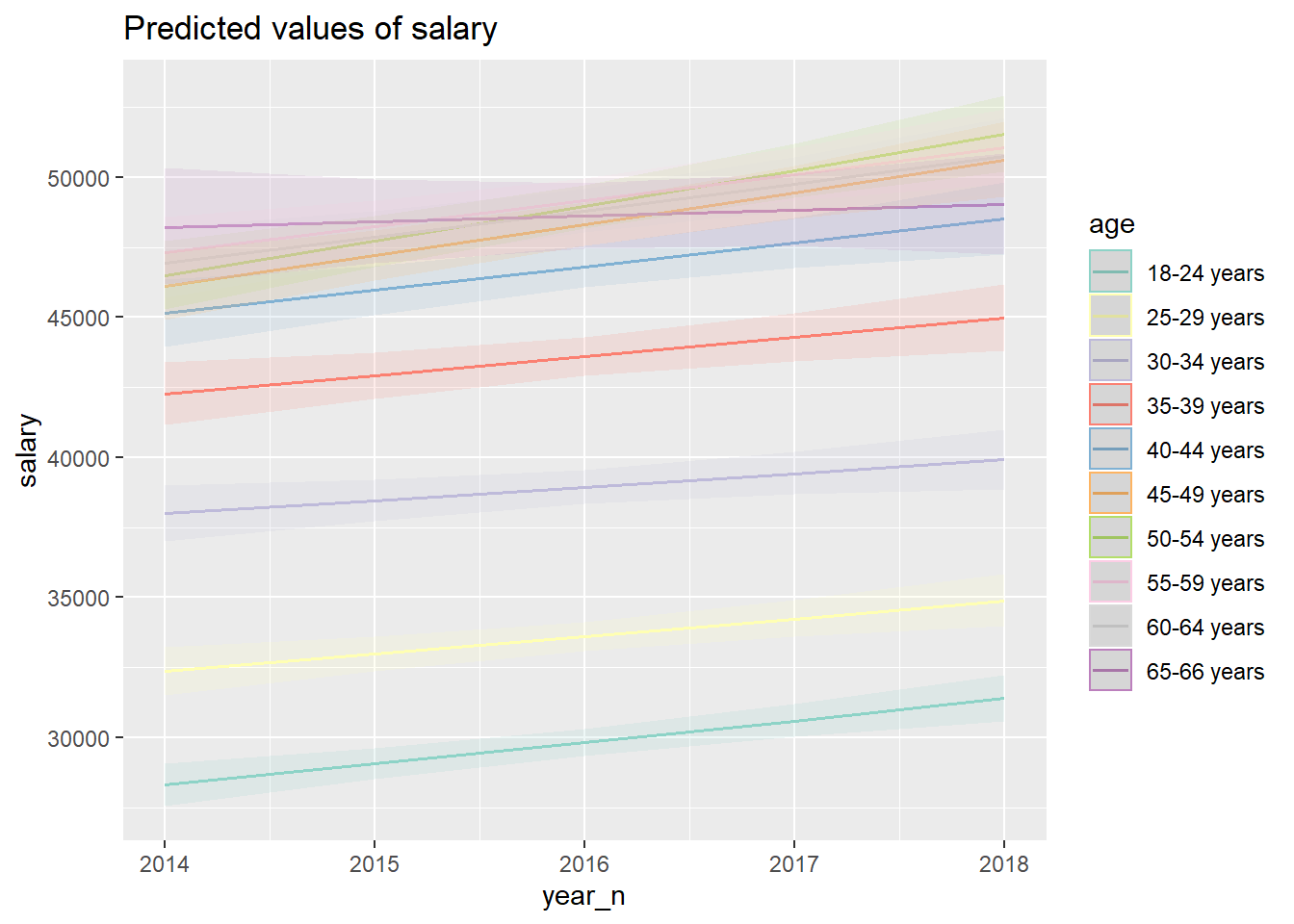
Figure 3: SSYK 214, Architects, engineers and related professionals, Year 2014 - 2018
plot(model, which = 1)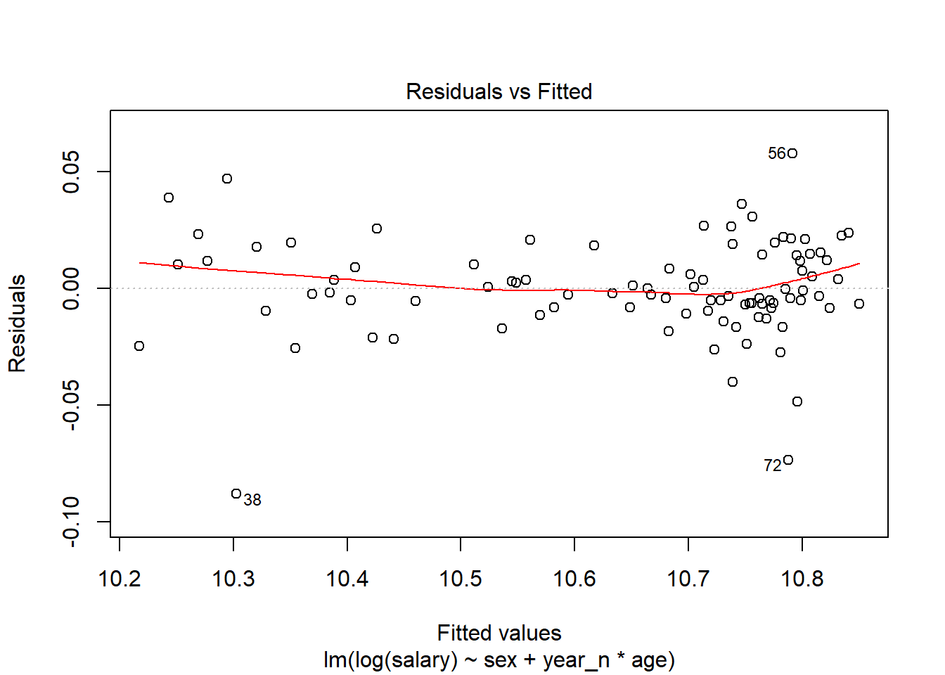
Figure 4: SSYK 214, Architects, engineers and related professionals, Year 2014 - 2018
model <- lm (log(salary) ~ sex + year_n * bs(age_n, knots = c(35, 50)), data = tb)

summary(model) %>%
  tidy() %>%
  knitr::kable(
  booktabs = TRUE,
caption = 'Summary from linear model fit')| term | estimate | std.error | statistic | p.value |
|---|---|---|---|---|
| (Intercept) | -42.2169094 | 10.4483489 | -4.0405340 | 0.0001206 |
| sexwomen | -0.0339907 | 0.0048836 | -6.9601677 | 0.0000000 |
| year_n | 0.0260513 | 0.0051827 | 5.0265834 | 0.0000029 |
| bs(age_n, knots = c(35, 50))1 | 15.9469335 | 23.8937700 | 0.6674097 | 0.5064075 |
| bs(age_n, knots = c(35, 50))2 | 37.3855896 | 23.7587981 | 1.5735472 | 0.1194903 |
| bs(age_n, knots = c(35, 50))3 | -8.1493593 | 25.1608613 | -0.3238903 | 0.7468559 |
| bs(age_n, knots = c(35, 50))4 | 8.6142351 | 22.3328612 | 0.3857202 | 0.7007151 |
| bs(age_n, knots = c(35, 50))5 | 37.8153976 | 18.0285162 | 2.0975324 | 0.0390644 |
| year_n:bs(age_n, knots = c(35, 50))1 | -0.0078854 | 0.0118521 | -0.6653159 | 0.5077385 |
| year_n:bs(age_n, knots = c(35, 50))2 | -0.0183302 | 0.0117851 | -1.5553743 | 0.1237557 |
| year_n:bs(age_n, knots = c(35, 50))3 | 0.0042939 | 0.0124805 | 0.3440519 | 0.7316989 |
| year_n:bs(age_n, knots = c(35, 50))4 | -0.0040248 | 0.0110776 | -0.3633240 | 0.7173094 |
| year_n:bs(age_n, knots = c(35, 50))5 | -0.0185161 | 0.0089421 | -2.0706713 | 0.0415743 |
summary(model)$adj.r.squared ## [1] 0.98315Anova(model, type = 2)## Anova Table (Type II tests)
##
## Response: log(salary)
## Sum Sq Df F value Pr(>F)
## sex 0.02618 1 48.4439 8.049e-10 ***
## year_n 0.06883 1 127.3747 < 2.2e-16 ***
## bs(age_n, knots = c(35, 50)) 2.81344 5 1041.2680 < 2.2e-16 ***
## year_n:bs(age_n, knots = c(35, 50)) 0.00445 5 1.6454 0.1574
## Residuals 0.04377 81
## ---
## Signif. codes: 0 '***' 0.001 '**' 0.01 '*' 0.05 '.' 0.1 ' ' 1plot_model(model, type = "pred", terms = c("age_n", "year_n"))## Model has log-transformed response. Back-transforming predictions to original response scale. Standard errors are still on the log-scale.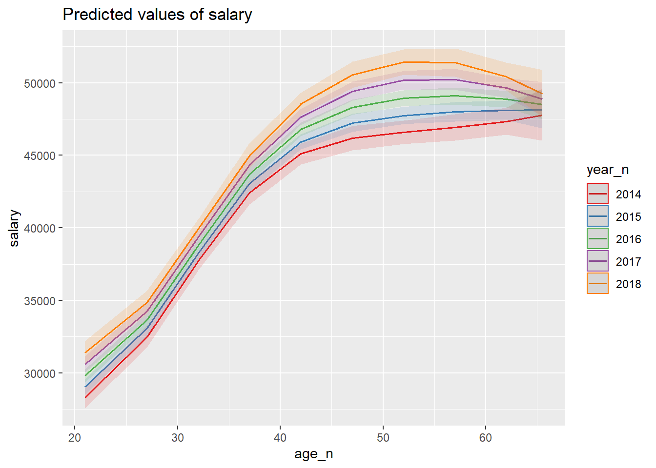
Figure 5: SSYK 214, Architects, engineers and related professionals, Year 2014 - 2018
plot(model, which = 1)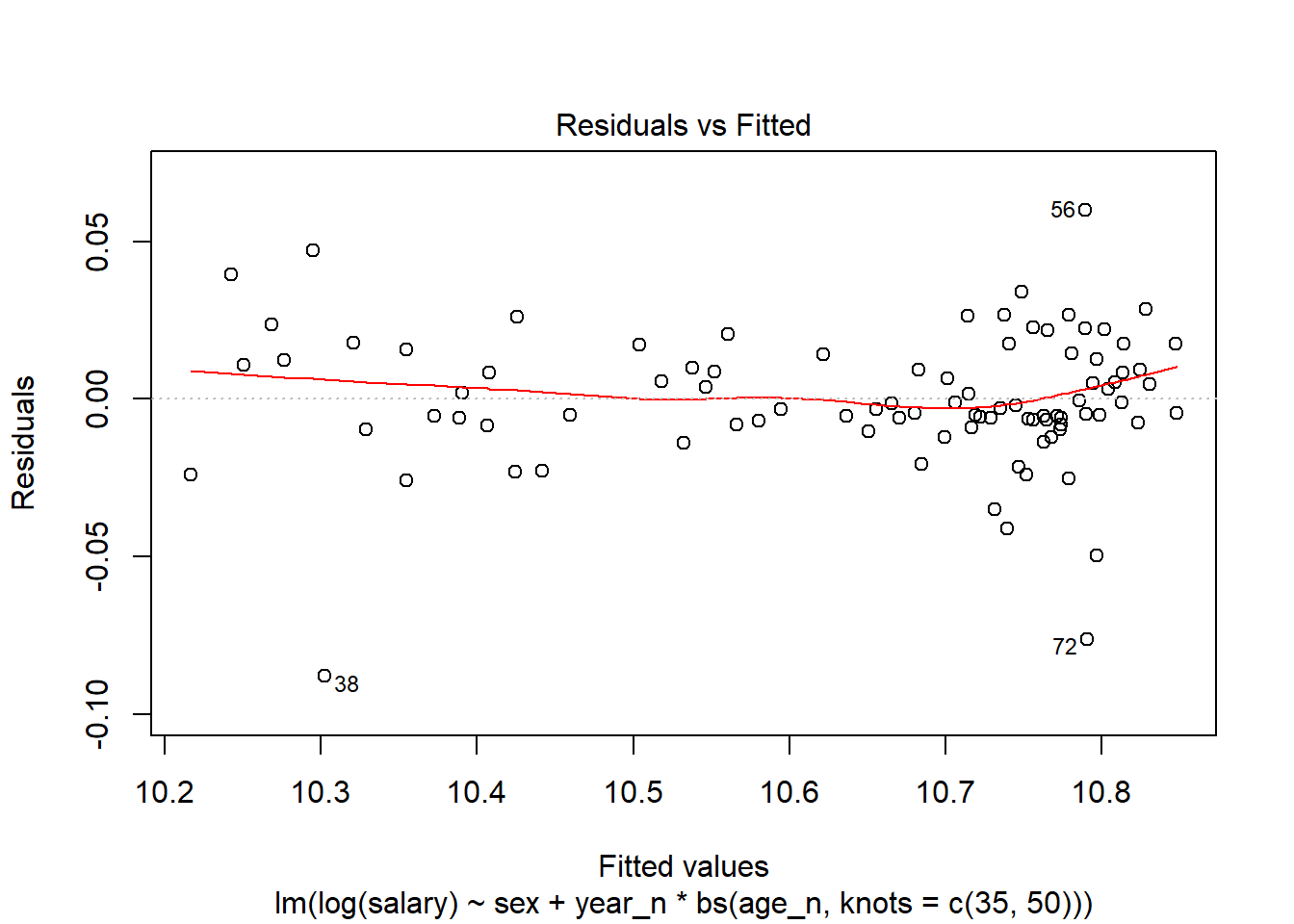
Figure 6: SSYK 214, Architects, engineers and related professionals, Year 2014 - 2018
Examine the interaction between gender and age. We can see that women have a significantly lower salary for the age groups 35-39 years, 45-49 years, 50-54 years, 55-59 years and 60-64 years.
The F-value from the Anova table for the interaction term between gender and age is 3,2 (Pr(>F) < 0.003564), sufficient for rejecting the null hypothesis that the interaction between gender and age has no effect on the salary holding year as constant.
model <- lm (log(salary) ~ year_n + sex * age, data = tb)

summary(model) %>%
  tidy() %>%
  knitr::kable(
  booktabs = TRUE,
caption = 'Summary from linear model fit')| term | estimate | std.error | statistic | p.value |
|---|---|---|---|---|
| (Intercept) | -28.2022208 | 3.2212924 | -8.7549396 | 0.0000000 |
| year_n | 0.0190896 | 0.0015979 | 11.9470190 | 0.0000000 |
| sexwomen | 0.0069060 | 0.0138839 | 0.4974127 | 0.6203728 |
| age25-29 years | 0.1287635 | 0.0138839 | 9.2743148 | 0.0000000 |
| age30-34 years | 0.2841357 | 0.0138839 | 20.4651381 | 0.0000000 |
| age35-39 years | 0.3994082 | 0.0138839 | 28.7677512 | 0.0000000 |
| age40-44 years | 0.4652656 | 0.0138839 | 33.5111890 | 0.0000000 |
| age45-49 years | 0.5076384 | 0.0138839 | 36.5631348 | 0.0000000 |
| age50-54 years | 0.5175734 | 0.0138839 | 37.2787098 | 0.0000000 |
| age55-59 years | 0.5389253 | 0.0138839 | 38.8166009 | 0.0000000 |
| age60-64 years | 0.5298153 | 0.0138839 | 38.1604449 | 0.0000000 |
| age65-66 years | 0.5054421 | 0.0147315 | 34.3102881 | 0.0000000 |
| sexwomen:age25-29 years | -0.0185979 | 0.0196348 | -0.9471913 | 0.3466242 |
| sexwomen:age30-34 years | -0.0342399 | 0.0196348 | -1.7438372 | 0.0853402 |
| sexwomen:age35-39 years | -0.0392078 | 0.0196348 | -1.9968533 | 0.0495192 |
| sexwomen:age40-44 years | -0.0290715 | 0.0196348 | -1.4806107 | 0.1429556 |
| sexwomen:age45-49 years | -0.0500604 | 0.0196348 | -2.5495786 | 0.0128556 |
| sexwomen:age50-54 years | -0.0435752 | 0.0196348 | -2.2192866 | 0.0295322 |
| sexwomen:age55-59 years | -0.0779734 | 0.0196348 | -3.9711888 | 0.0001643 |
| sexwomen:age60-64 years | -0.0742603 | 0.0196348 | -3.7820779 | 0.0003131 |
summary(model)$adj.r.squared ## [1] 0.9849736Anova(model, type = 2)## Note: model has aliased coefficients
## sums of squares computed by model comparison## Anova Table (Type II tests)
##
## Response: log(salary)
## Sum Sq Df F value Pr(>F)
## year_n 0.06878 1 142.7313 < 2.2e-16 ***
## sex 0.02581 1 53.5620 2.492e-10 ***
## age 2.81366 9 648.7344 < 2.2e-16 ***
## sex:age 0.01234 8 3.2006 0.003564 **
## Residuals 0.03566 74
## ---
## Signif. codes: 0 '***' 0.001 '**' 0.01 '*' 0.05 '.' 0.1 ' ' 1plot_model(model, type = "pred", terms = c("age", "sex"))## Warning in predict.lm(model, newdata = fitfram, type = "response", se.fit =
## se, : prediction from a rank-deficient fit may be misleading## Model has log-transformed response. Back-transforming predictions to original response scale. Standard errors are still on the log-scale.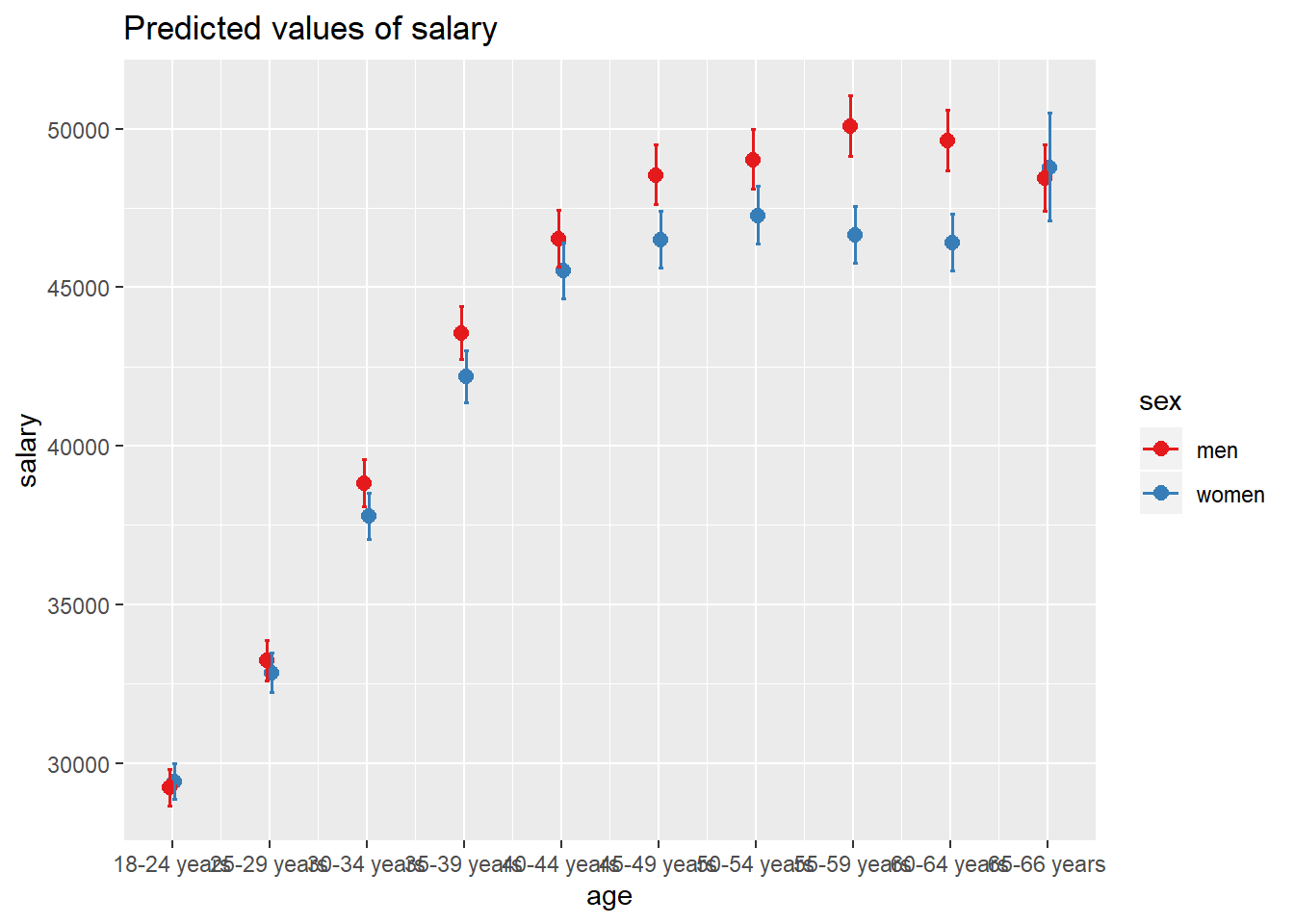
Figure 7: SSYK 214, Architects, engineers and related professionals, Year 2014 - 2018
plot(model, which = 1)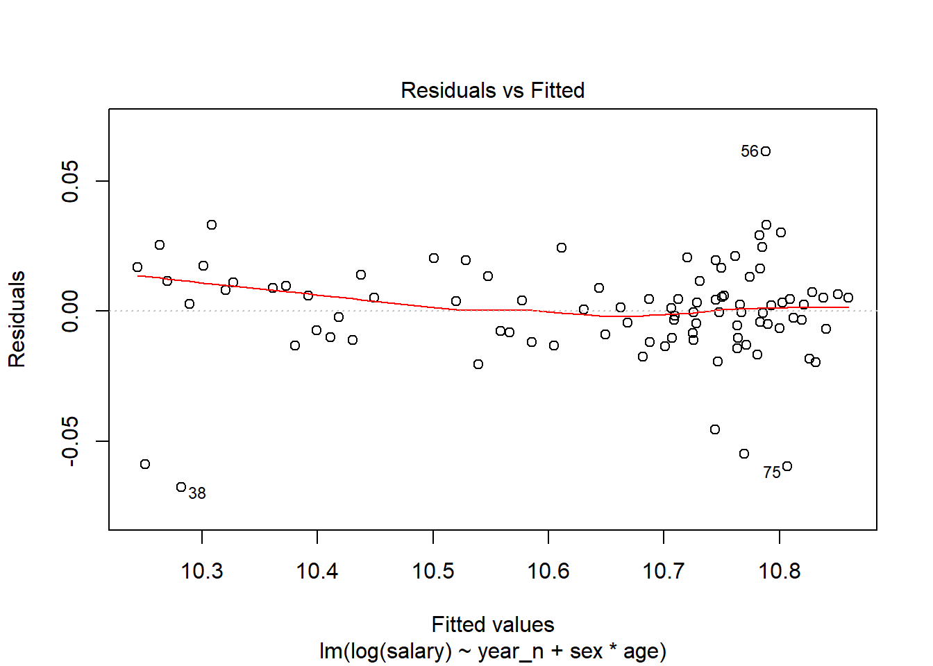
Figure 8: SSYK 214, Architects, engineers and related professionals, Year 2014 - 2018
tb[75,]## Source: local data frame [1 x 9]
## Groups: <by row>
##
## # A tibble: 1 x 9
## `occuptional (SSYK 2012~ age sex year salary year_n age_l age_h age_n
## <chr> <chr> <chr> <chr> <dbl> <dbl> <int> <int> <dbl>
## 1 214 Engineering professi~ 65-66 y~ men 2017 46500 2017 65 66 65.5model <- lm (log(salary) ~ year_n + sex * bs(age_n, knots = c(35, 50)), data = tb)
summary(model) %>%
tidy() %>%
knitr::kable(
booktabs = TRUE,
caption = 'Summary from linear model fit')| term | estimate | std.error | statistic | p.value |
|---|---|---|---|---|
| (Intercept) | -28.2038536 | 3.1195378 | -9.0410359 | 0.0000000 |
| year_n | 0.0190902 | 0.0015474 | 12.3371071 | 0.0000000 |
| sexwomen | 0.0071007 | 0.0134078 | 0.5295958 | 0.5978408 |
| bs(age_n, knots = c(35, 50))1 | 0.0569146 | 0.0216453 | 2.6294148 | 0.0102324 |
| bs(age_n, knots = c(35, 50))2 | 0.4595799 | 0.0214465 | 21.4291344 | 0.0000000 |
| bs(age_n, knots = c(35, 50))3 | 0.5131788 | 0.0225545 | 22.7528180 | 0.0000000 |
| bs(age_n, knots = c(35, 50))4 | 0.5585990 | 0.0195443 | 28.5811988 | 0.0000000 |
| bs(age_n, knots = c(35, 50))5 | 0.5056993 | 0.0139459 | 36.2613732 | 0.0000000 |
| sexwomen:bs(age_n, knots = c(35, 50))1 | -0.0156019 | 0.0309691 | -0.5037899 | 0.6157765 |
| sexwomen:bs(age_n, knots = c(35, 50))2 | -0.0520644 | 0.0314890 | -1.6534151 | 0.1021172 |
| sexwomen:bs(age_n, knots = c(35, 50))3 | -0.0173455 | 0.0347256 | -0.4995018 | 0.6187800 |
| sexwomen:bs(age_n, knots = c(35, 50))4 | -0.1083142 | 0.0346022 | -3.1302674 | 0.0024289 |
| sexwomen:bs(age_n, knots = c(35, 50))5 | -0.0509037 | 0.0386819 | -1.3159563 | 0.1919009 |
summary(model)$adj.r.squared ## [1] 0.9859063Anova(model, type = 2)## Anova Table (Type II tests)
##
## Response: log(salary)
## Sum Sq Df F value Pr(>F)
## year_n 0.06880 1 152.2042 < 2.2e-16 ***
## sex 0.02612 1 57.7814 4.558e-11 ***
## bs(age_n, knots = c(35, 50)) 2.81344 5 1244.9030 < 2.2e-16 ***
## sex:bs(age_n, knots = c(35, 50)) 0.01161 5 5.1354 0.0003844 ***
## Residuals 0.03661 81
## ---
## Signif. codes: 0 '***' 0.001 '**' 0.01 '*' 0.05 '.' 0.1 ' ' 1plot_model(model, type = "pred", terms = c("age_n", "sex"))## Model has log-transformed response. Back-transforming predictions to original response scale. Standard errors are still on the log-scale.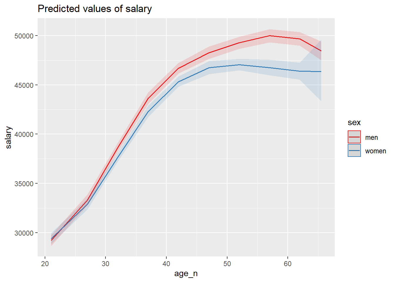
Figure 9: SSYK 214, Architects, engineers and related professionals, Year 2014 - 2018
plot(model, which = 1)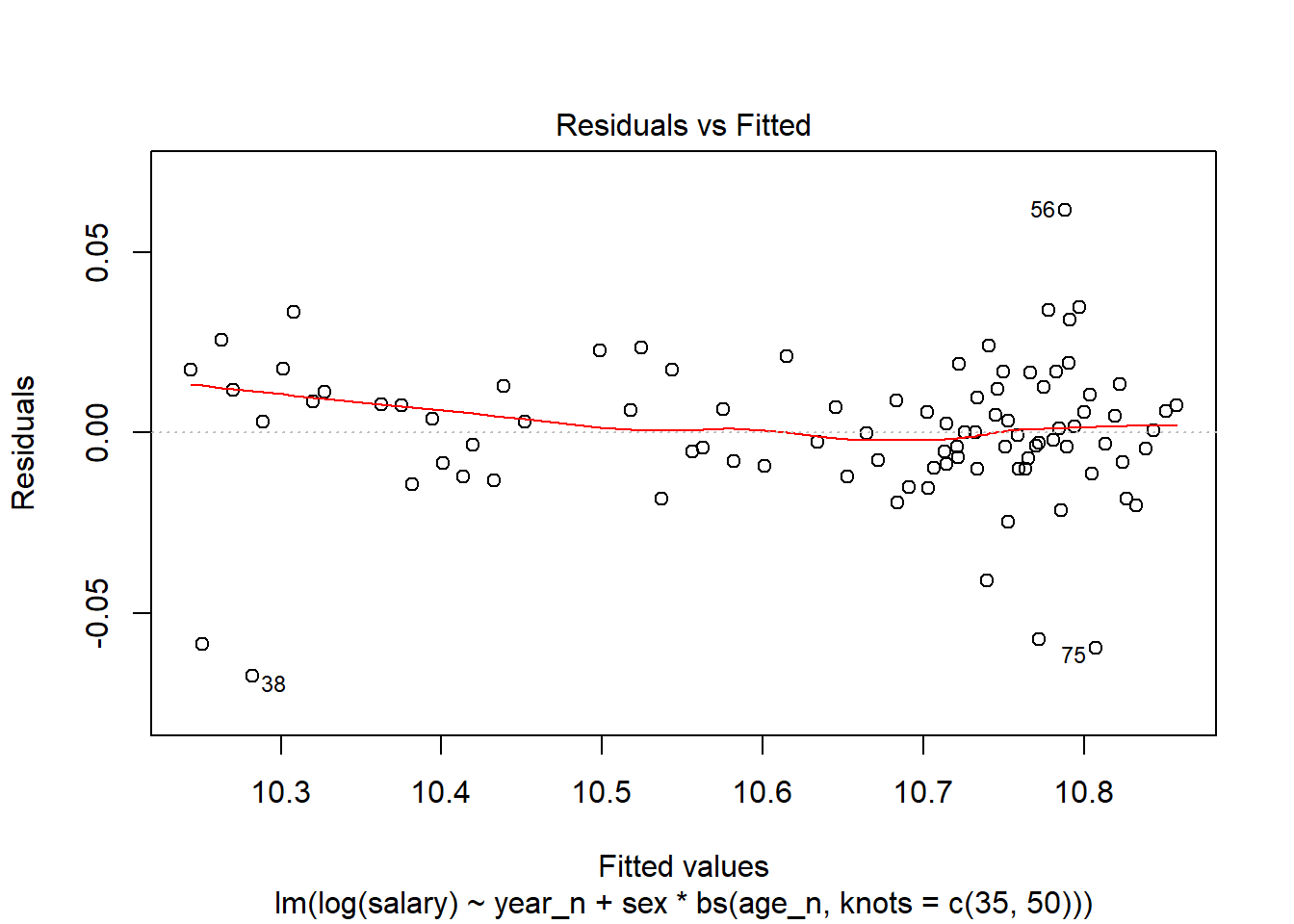
Figure 10: SSYK 214, Architects, engineers and related professionals, Year 2014 - 2018
Examine the interaction between gender and year. Both the model with categorical predictors and the model with continuous predictors indicates that women’s salaries increase more than men’s salaries.
The F-value from the Anova table for the interaction term between gender and year is 3,1 (Pr(>F) < 0.08053), with 90 % significance we can reject the null hypothesis that the interaction between gender and year has no effect on the salary holding age as constant.
model <- lm (log(salary) ~ year_n * sex + age, data = tb)

summary(model) %>%
  tidy() %>%
  knitr::kable(
  booktabs = TRUE,
caption = 'Summary from linear model fit')| term | estimate | std.error | statistic | p.value |
|---|---|---|---|---|
| (Intercept) | -22.2600278 | 4.8457687 | -4.593704 | 0.0000158 |
| year_n | 0.0161522 | 0.0024037 | 6.719863 | 0.0000000 |
| sexwomen | -12.4532110 | 7.0175325 | -1.774585 | 0.0797236 |
| age25-29 years | 0.1194646 | 0.0106821 | 11.183664 | 0.0000000 |
| age30-34 years | 0.2670157 | 0.0106821 | 24.996646 | 0.0000000 |
| age35-39 years | 0.3798043 | 0.0106821 | 35.555336 | 0.0000000 |
| age40-44 years | 0.4507298 | 0.0106821 | 42.195020 | 0.0000000 |
| age45-49 years | 0.4826082 | 0.0106821 | 45.179312 | 0.0000000 |
| age50-54 years | 0.4957858 | 0.0106821 | 46.412928 | 0.0000000 |
| age55-59 years | 0.4999386 | 0.0106821 | 46.801692 | 0.0000000 |
| age60-64 years | 0.4926852 | 0.0106821 | 46.122664 | 0.0000000 |
| age65-66 years | 0.4857883 | 0.0143662 | 33.814759 | 0.0000000 |
| year_n:sexwomen | 0.0061604 | 0.0034809 | 1.769759 | 0.0805306 |
summary(model)$adj.r.squared ## [1] 0.9822101Anova(model, type = 2)## Anova Table (Type II tests)
##
## Response: log(salary)
## Sum Sq Df F value Pr(>F)
## year_n 0.06878 1 120.559 < 2.2e-16 ***
## sex 0.02581 1 45.242 2.266e-09 ***
## age 2.81430 9 548.084 < 2.2e-16 ***
## year_n:sex 0.00179 1 3.132 0.08053 .
## Residuals 0.04621 81
## ---
## Signif. codes: 0 '***' 0.001 '**' 0.01 '*' 0.05 '.' 0.1 ' ' 1plot_model(model, type = "pred", terms = c("year_n", "sex"))## Model has log-transformed response. Back-transforming predictions to original response scale. Standard errors are still on the log-scale.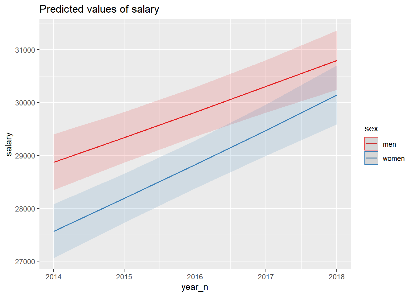
Figure 11: SSYK 214, Architects, engineers and related professionals, Year 2014 - 2018
model <- lm (log(salary) ~ year_n * sex + bs(age_n, knots = c(35, 50)), data = tb)

summary(model) %>%
  tidy() %>%
  knitr::kable(
  booktabs = TRUE,
caption = 'Summary from linear model fit')| term | estimate | std.error | statistic | p.value |
|---|---|---|---|---|
| (Intercept) | -22.2810163 | 4.7408239 | -4.699819 | 0.0000099 |
| year_n | 0.0161625 | 0.0023516 | 6.872990 | 0.0000000 |
| sexwomen | -12.4325740 | 6.8662746 | -1.810672 | 0.0737248 |
| bs(age_n, knots = c(35, 50))1 | 0.0497887 | 0.0168608 | 2.952920 | 0.0040694 |
| bs(age_n, knots = c(35, 50))2 | 0.4323307 | 0.0167836 | 25.759071 | 0.0000000 |
| bs(age_n, knots = c(35, 50))3 | 0.5064797 | 0.0178110 | 28.436385 | 0.0000000 |
| bs(age_n, knots = c(35, 50))4 | 0.5014488 | 0.0159182 | 31.501692 | 0.0000000 |
| bs(age_n, knots = c(35, 50))5 | 0.4850317 | 0.0132343 | 36.649526 | 0.0000000 |
| year_n:sexwomen | 0.0061501 | 0.0034059 | 1.805728 | 0.0745008 |
summary(model)$adj.r.squared ## [1] 0.9829655Anova(model, type = 2)## Anova Table (Type II tests)
##
## Response: log(salary)
## Sum Sq Df F value Pr(>F)
## year_n 0.06883 1 125.9950 < 2.2e-16 ***
## sex 0.02612 1 47.8063 8.182e-10 ***
## bs(age_n, knots = c(35, 50)) 2.81407 5 1030.2198 < 2.2e-16 ***
## year_n:sex 0.00178 1 3.2607 0.0745 .
## Residuals 0.04644 85
## ---
## Signif. codes: 0 '***' 0.001 '**' 0.01 '*' 0.05 '.' 0.1 ' ' 1plot_model(model, type = "pred", terms = c("year_n", "sex"))## Model has log-transformed response. Back-transforming predictions to original response scale. Standard errors are still on the log-scale.
Figure 12: SSYK 214, Architects, engineers and related professionals, Year 2014 - 2018
Examine the interaction between year, gender and age. It’s becoming a bit difficult to make any significant predictions about the interactions from the model, the data is not sufficiently large, the degrees of freedom has been reduced from 82 in the model with no interaction terms to 56.
The following interaction terms are significant to 90 %.
year_n:sexwomen
sexwomen:age35-39 years
year_n:sexwomen:age35-39 years
In the graph below you can that the salaries for men in the age group 35-39 years has increased more than for women.
The F-value from the Anova table for the interaction term between gender and age is 3,3 (Pr(>F) < 0.00373), sufficient for rejecting the null hypothesis that the interaction between gender and age has no effect on the salary holding year as constant.
model <- lm (log(salary) ~ year_n * sex * age, data = tb)

summary(model) %>%
  tidy() %>%
  knitr::kable(
  booktabs = TRUE,
caption = 'Summary from linear model fit')| term | estimate | std.error | statistic | p.value |
|---|---|---|---|---|
| (Intercept) | -23.0500250 | 13.7844076 | -1.6721810 | 0.1000676 |
| year_n | 0.0165340 | 0.0068375 | 2.4181290 | 0.0188783 |
| sexwomen | -37.6245789 | 19.4940962 | -1.9300499 | 0.0586714 |
| age25-29 years | 0.3057247 | 19.4940962 | 0.0156829 | 0.9875431 |
| age30-34 years | 13.4212323 | 19.4940962 | 0.6884768 | 0.4939950 |
| age35-39 years | -6.4835219 | 19.4940962 | -0.3325890 | 0.7406864 |
| age40-44 years | -4.3559249 | 19.4940962 | -0.2234484 | 0.8239997 |
| age45-49 years | -8.7690292 | 19.4940962 | -0.4498300 | 0.6545695 |
| age50-54 years | -0.8787263 | 19.4940962 | -0.0450765 | 0.9642067 |
| age55-59 years | -6.3664653 | 19.4940962 | -0.3265843 | 0.7451998 |
| age60-64 years | 2.4331505 | 19.4940962 | 0.1248147 | 0.9011172 |
| age65-66 years | 25.2691238 | 20.1796414 | 1.2522088 | 0.2156985 |
| year_n:sexwomen | 0.0186664 | 0.0096697 | 1.9304047 | 0.0586265 |
| year_n:age25-29 years | -0.0000878 | 0.0096697 | -0.0090777 | 0.9927894 |
| year_n:age30-34 years | -0.0065164 | 0.0096697 | -0.6739015 | 0.5031462 |
| year_n:age35-39 years | 0.0034142 | 0.0096697 | 0.3530778 | 0.7253558 |
| year_n:age40-44 years | 0.0023915 | 0.0096697 | 0.2473155 | 0.8055686 |
| year_n:age45-49 years | 0.0046015 | 0.0096697 | 0.4758707 | 0.6360177 |
| year_n:age50-54 years | 0.0006926 | 0.0096697 | 0.0716268 | 0.9431541 |
| year_n:age55-59 years | 0.0034253 | 0.0096697 | 0.3542299 | 0.7244970 |
| year_n:age60-64 years | -0.0009441 | 0.0096697 | -0.0976365 | 0.9225696 |
| year_n:age65-66 years | -0.0122817 | 0.0100091 | -1.2270593 | 0.2249341 |
| sexwomen:age25-29 years | 28.1128665 | 27.5688152 | 1.0197343 | 0.3122398 |
| sexwomen:age30-34 years | 28.1928073 | 27.5688152 | 1.0226340 | 0.3108784 |
| sexwomen:age35-39 years | 54.9538639 | 27.5688152 | 1.9933343 | 0.0511051 |
| sexwomen:age40-44 years | 41.2101760 | 27.5688152 | 1.4948113 | 0.1405778 |
| sexwomen:age45-49 years | 29.0456019 | 27.5688152 | 1.0535673 | 0.2966058 |
| sexwomen:age50-54 years | 3.1386820 | 27.5688152 | 0.1138490 | 0.9097647 |
| sexwomen:age55-59 years | 41.1408823 | 27.5688152 | 1.4922978 | 0.1412337 |
| sexwomen:age60-64 years | 21.7389989 | 27.5688152 | 0.7885358 | 0.4337089 |
| year_n:sexwomen:age25-29 years | -0.0139541 | 0.0136750 | -1.0204092 | 0.3119226 |
| year_n:sexwomen:age30-34 years | -0.0140015 | 0.0136750 | -1.0238762 | 0.3102964 |
| year_n:sexwomen:age35-39 years | -0.0272783 | 0.0136750 | -1.9947569 | 0.0509451 |
| year_n:sexwomen:age40-44 years | -0.0204560 | 0.0136750 | -1.4958662 | 0.1403033 |
| year_n:sexwomen:age45-49 years | -0.0144324 | 0.0136750 | -1.0553834 | 0.2957821 |
| year_n:sexwomen:age50-54 years | -0.0015785 | 0.0136750 | -0.1154296 | 0.9085175 |
| year_n:sexwomen:age55-59 years | -0.0204459 | 0.0136750 | -1.4951265 | 0.1404958 |
| year_n:sexwomen:age60-64 years | -0.0108201 | 0.0136750 | -0.7912297 | 0.4321485 |
summary(model)$adj.r.squared ## [1] 0.9854223Anova(model, type = 2)## Note: model has aliased coefficients
## sums of squares computed by model comparison## Anova Table (Type II tests)
##
## Response: log(salary)
## Sum Sq Df F value Pr(>F)
## year_n 0.06878 1 147.1250 < 2.2e-16 ***
## sex 0.02581 1 55.2108 6.727e-10 ***
## age 2.81430 9 668.8557 < 2.2e-16 ***
## year_n:sex 0.00113 1 2.4097 0.12622
## year_n:age 0.00460 9 1.0927 0.38295
## sex:age 0.01234 8 3.2991 0.00373 **
## year_n:sex:age 0.00310 8 0.8277 0.58192
## Residuals 0.02618 56
## ---
## Signif. codes: 0 '***' 0.001 '**' 0.01 '*' 0.05 '.' 0.1 ' ' 1plot_model(model, type = "pred", terms = c("year_n", "age", "sex"))## Warning in predict.lm(model, newdata = fitfram, type = "response", se.fit =
## se, : prediction from a rank-deficient fit may be misleading## Model has log-transformed response. Back-transforming predictions to original response scale. Standard errors are still on the log-scale.## Warning in RColorBrewer::brewer.pal(n, pal): n too large, allowed maximum for palette Set1 is 9
## Returning the palette you asked for with that many colors## Warning: Removed 10 rows containing missing values (geom_path).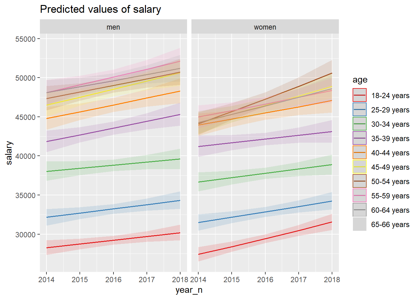
Figure 13: SSYK 214, Architects, engineers and related professionals, Year 2014 - 2018
plot(model, which = 1)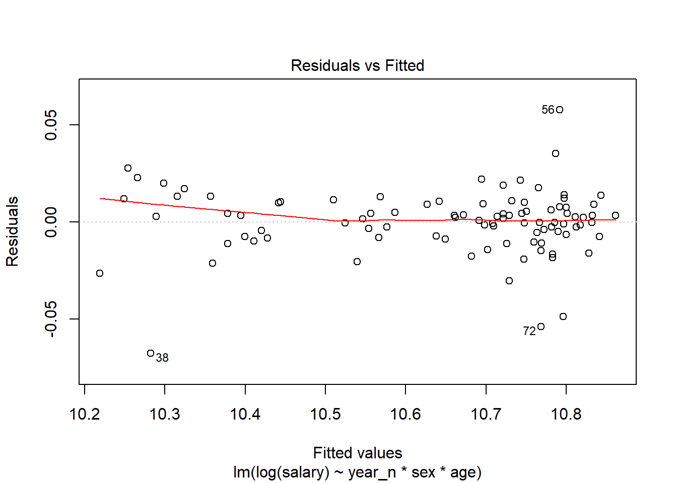
Figure 14: SSYK 214, Architects, engineers and related professionals, Year 2014 - 2018
model <- lm (log(salary) ~ year_n * sex * bs(age_n, knots = c(35, 50)), data = tb)

summary(model) %>%
  tidy() %>%
  knitr::kable(
  booktabs = TRUE,
caption = 'Summary from linear model fit')| term | estimate | std.error | statistic | p.value |
|---|---|---|---|---|
| (Intercept) | -24.0868942 | 12.7931370 | -1.8827981 | 0.0638836 |
| year_n | 0.0170481 | 0.0063458 | 2.6865147 | 0.0090115 |
| sexwomen | -35.9593922 | 18.0942402 | -1.9873392 | 0.0507987 |
| bs(age_n, knots = c(35, 50))1 | 13.5471021 | 29.2057808 | 0.4638500 | 0.6441944 |
| bs(age_n, knots = c(35, 50))2 | -3.5308622 | 28.9253132 | -0.1220682 | 0.9031947 |
| bs(age_n, knots = c(35, 50))3 | -3.0003750 | 30.3944067 | -0.0987147 | 0.9216469 |
| bs(age_n, knots = c(35, 50))4 | -10.6818355 | 26.2596260 | -0.4067779 | 0.6854122 |
| bs(age_n, knots = c(35, 50))5 | 24.6956649 | 18.4012753 | 1.3420627 | 0.1839126 |
| year_n:sexwomen | 0.0178405 | 0.0089753 | 1.9877332 | 0.0507540 |
| year_n:bs(age_n, knots = c(35, 50))1 | -0.0066913 | 0.0144870 | -0.4618860 | 0.6455954 |
| year_n:bs(age_n, knots = c(35, 50))2 | 0.0019790 | 0.0143478 | 0.1379286 | 0.8906928 |
| year_n:bs(age_n, knots = c(35, 50))3 | 0.0017435 | 0.0150765 | 0.1156429 | 0.9082666 |
| year_n:bs(age_n, knots = c(35, 50))4 | 0.0055746 | 0.0130255 | 0.4279781 | 0.6699809 |
| year_n:bs(age_n, knots = c(35, 50))5 | -0.0119974 | 0.0091271 | -1.3144829 | 0.1929745 |
| sexwomen:bs(age_n, knots = c(35, 50))1 | -3.0882433 | 41.7901518 | -0.0738988 | 0.9413017 |
| sexwomen:bs(age_n, knots = c(35, 50))2 | 96.0533158 | 42.4835588 | 2.2609527 | 0.0268729 |
| sexwomen:bs(age_n, knots = c(35, 50))3 | -33.3604447 | 46.8350731 | -0.7122962 | 0.4786489 |
| sexwomen:bs(age_n, knots = c(35, 50))4 | 73.5641700 | 46.6314260 | 1.5775664 | 0.1191741 |
| sexwomen:bs(age_n, knots = c(35, 50))5 | -29.6631727 | 52.0527929 | -0.5698671 | 0.5705923 |
| year_n:sexwomen:bs(age_n, knots = c(35, 50))1 | 0.0015239 | 0.0207292 | 0.0735146 | 0.9416063 |
| year_n:sexwomen:bs(age_n, knots = c(35, 50))2 | -0.0476709 | 0.0210732 | -2.2621610 | 0.0267943 |
| year_n:sexwomen:bs(age_n, knots = c(35, 50))3 | 0.0165386 | 0.0232316 | 0.7118987 | 0.4788935 |
| year_n:sexwomen:bs(age_n, knots = c(35, 50))4 | -0.0365429 | 0.0231306 | -1.5798519 | 0.1186493 |
| year_n:sexwomen:bs(age_n, knots = c(35, 50))5 | 0.0146870 | 0.0258196 | 0.5688315 | 0.5712911 |
summary(model)$adj.r.squared ## [1] 0.9873689Anova(model, type = 2)## Anova Table (Type II tests)
##
## Response: log(salary)
## Sum Sq Df F value Pr(>F)
## year_n 0.06880 1 169.8286 < 2.2e-16 ***
## sex 0.03780 6 15.5511 3.011e-11 ***
## bs(age_n, knots = c(35, 50)) 2.82569 10 697.5506 < 2.2e-16 ***
## year_n:sex 0.00126 1 3.1090 0.0822248 .
## year_n:bs(age_n, knots = c(35, 50)) 0.00394 5 1.9452 0.0977419 .
## sex:bs(age_n, knots = c(35, 50)) 0.01163 5 5.7405 0.0001702 ***
## year_n:sex:bs(age_n, knots = c(35, 50)) 0.00253 5 1.2489 0.2958798
## Residuals 0.02836 70
## ---
## Signif. codes: 0 '***' 0.001 '**' 0.01 '*' 0.05 '.' 0.1 ' ' 1plot_model(model, type = "pred", terms = c("age_n", "year_n", "sex"))## Model has log-transformed response. Back-transforming predictions to original response scale. Standard errors are still on the log-scale.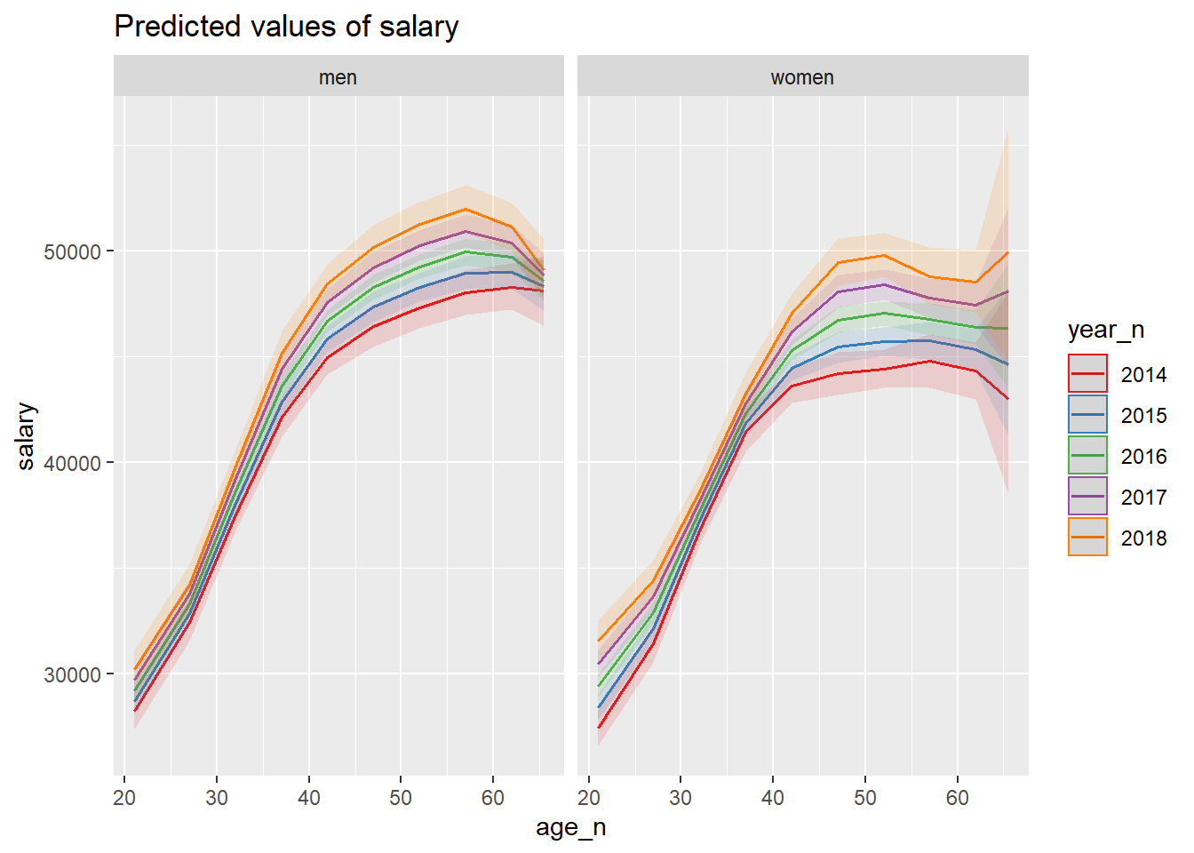
Figure 15: SSYK 214, Architects, engineers and related professionals, Year 2014 - 2018
plot(model, which = 1)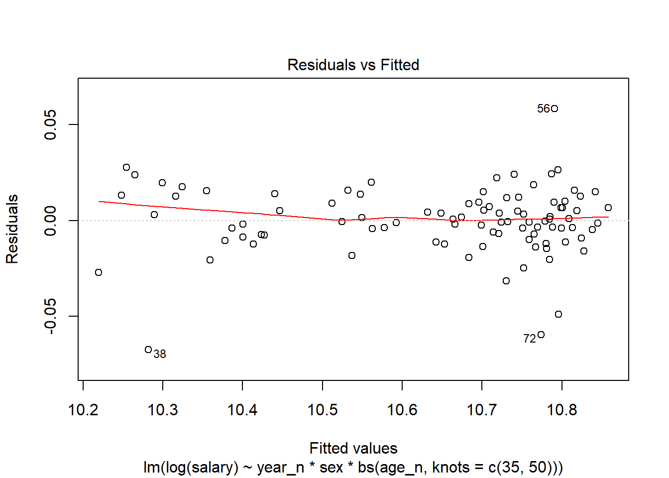
Figure 16: SSYK 214, Architects, engineers and related professionals, Year 2014 - 2018
Average basic salary, monthly salary and women´s salary as a percentage of men´s salary by sector, occupational group (SSYK 2012), gender and educational level (SUN). Year 2014 - 2018 Monthly salary All sectors
We expect that gender is an important factor in salaries. As a null hypothesis, we assume that the interaction between gender and education is not related to the salary and examine if we can reject this hypothesis with the data from Statistics Sweden.
tb <- readfile("000000CY.csv") %>%
  filter(`occuptional  (SSYK 2012)` == "214 Engineering professionals") %>%
  mutate(edulevel = `level of education`)

numedulevel <- read.csv("edulevel.csv")

tbnum <- tb %>%
  right_join(numedulevel, by = c("level of education" = "level.of.education")) %>%
  filter(!is.na(eduyears))
## Warning: Column `level of education`/`level.of.education` joining character
## vector and factor, coercing into character vectornumedulevel %>%
knitr::kable(
booktabs = TRUE,
caption = 'Initial approach, length of education') | level.of.education | eduyears |
|---|---|
| primary and secondary education 9-10 years (ISCED97 2) | 9 |
| upper secondary education, 2 years or less (ISCED97 3C) | 11 |
| upper secondary education 3 years (ISCED97 3A) | 12 |
| post-secondary education, less than 3 years (ISCED97 4+5B) | 14 |
| post-secondary education 3 years or more (ISCED97 5A) | 15 |
| post-graduate education (ISCED97 6) | 19 |
| no information about level of educational attainment | NA |
tb %>%
  ggplot () +
    geom_point (mapping = aes(x = year_n,y = salary, colour = `level of education`, shape = sex)) +
  labs(
    x = "Year",
    y = "Salary (SEK/month)"
  )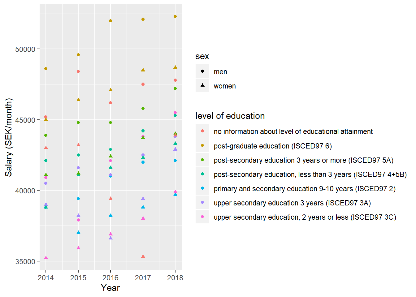
Figure 17: SSYK 214, Architects, engineers and related professionals, Year 2014 - 2018
model <- lm (log(salary) ~ year_n + sex + edulevel, data = tbnum)

summary(model) %>%
  tidy() %>%
  knitr::kable(
  booktabs = TRUE,
caption = 'Summary from linear model fit')| term | estimate | std.error | statistic | p.value |
|---|---|---|---|---|
| (Intercept) | -34.8741818 | 4.5648337 | -7.639749 | 0 |
| year_n | 0.0226738 | 0.0022643 | 10.013413 | 0 |
| sexwomen | -0.0743114 | 0.0063438 | -11.713990 | 0 |
| edulevelpost-secondary education 3 years or more (ISCED97 5A) | -0.1104356 | 0.0108816 | -10.148796 | 0 |
| edulevelpost-secondary education, less than 3 years (ISCED97 4+5B) | -0.1446573 | 0.0108816 | -13.293700 | 0 |
| edulevelprimary and secondary education 9-10 years (ISCED97 2) | -0.2207500 | 0.0111971 | -19.714892 | 0 |
| edulevelupper secondary education 3 years (ISCED97 3A) | -0.1898866 | 0.0108816 | -17.450172 | 0 |
| edulevelupper secondary education, 2 years or less (ISCED97 3C) | -0.2155065 | 0.0108816 | -19.804583 | 0 |
summary(model)$adj.r.squared ## [1] 0.9311952Anova(model, type = 2)## Anova Table (Type II tests)
##
## Response: log(salary)
## Sum Sq Df F value Pr(>F)
## year_n 0.05936 1 100.27 1.232e-13 ***
## sex 0.08124 1 137.22 4.476e-16 ***
## edulevel 0.34338 5 116.00 < 2.2e-16 ***
## Residuals 0.03019 51
## ---
## Signif. codes: 0 '***' 0.001 '**' 0.01 '*' 0.05 '.' 0.1 ' ' 1plot(model, which = 1)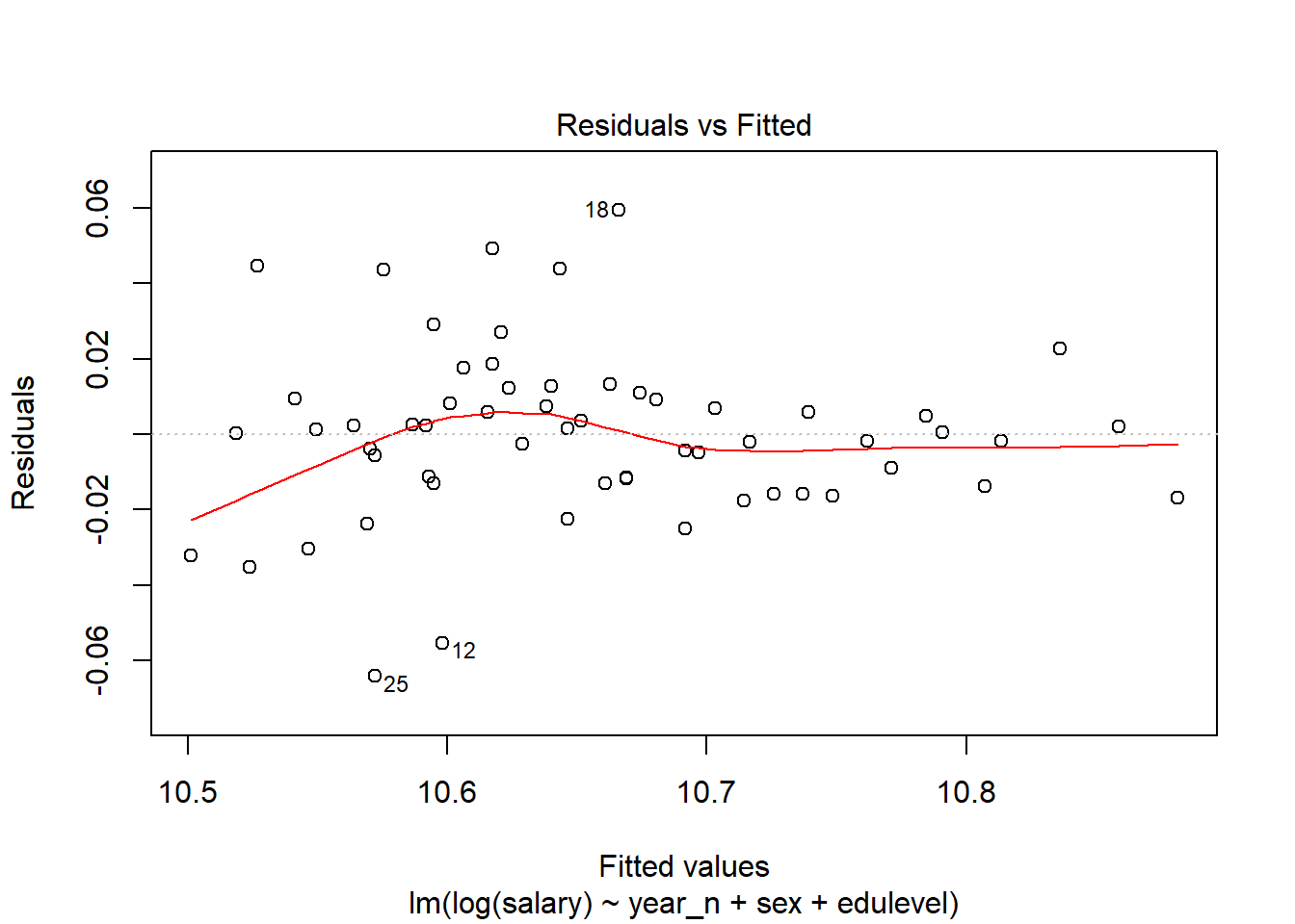
Figure 18: SSYK 214, Architects, engineers and related professionals, Year 2014 - 2018
tb[20,]## # A tibble: 1 x 8
## sector `occuptional (~ sex `level of educat~ year salary year_n edulevel
## <chr> <chr> <chr> <chr> <chr> <dbl> <dbl> <chr>
## 1 0 all ~ 214 Engineering~ men no information a~ 2015 48400 2015 no infor~tb[41,]## # A tibble: 1 x 8
## sector `occuptional (~ sex `level of educat~ year salary year_n edulevel
## <chr> <chr> <chr> <chr> <chr> <dbl> <dbl> <chr>
## 1 0 all ~ 214 Engineering~ women no information a~ 2016 39400 2016 no infor~tb[55,]## # A tibble: 1 x 8
## sector `occuptional (~ sex `level of educat~ year salary year_n edulevel
## <chr> <chr> <chr> <chr> <chr> <dbl> <dbl> <chr>
## 1 0 all ~ 214 Engineering~ women no information a~ 2017 35300 2017 no infor~We start by examining the interaction between year and education. The salaries for the education upper secondary education, 2 years or less increase more than other educations during the time period 2014-2018, however, this can not be shown with 95% significance from this data.
model <- lm(log(salary) ~ sex + year_n * edulevel, data = tbnum)

summary(model) %>%
  tidy() %>%
  knitr::kable(
  booktabs = TRUE,
caption = 'Summary from linear model fit')| term | estimate | std.error | statistic | p.value |
|---|---|---|---|---|
| (Intercept) | -29.3041153 | 10.9645273 | -2.6726291 | 0.0103775 |
| sexwomen | -0.0743499 | 0.0063563 | -11.6971241 | 0.0000000 |
| year_n | 0.0199109 | 0.0054388 | 3.6609245 | 0.0006464 |
| edulevelpost-secondary education 3 years or more (ISCED97 5A) | 3.5092165 | 15.5061826 | 0.2263108 | 0.8219623 |
| edulevelpost-secondary education, less than 3 years (ISCED97 4+5B) | -3.7498523 | 15.5061826 | -0.2418295 | 0.8099871 |
| edulevelprimary and secondary education 9-10 years (ISCED97 2) | -6.8196567 | 16.6031078 | -0.4107458 | 0.6831661 |
| edulevelupper secondary education 3 years (ISCED97 3A) | -0.3311115 | 15.5061826 | -0.0213535 | 0.9830560 |
| edulevelupper secondary education, 2 years or less (ISCED97 3C) | -27.1431543 | 15.5061826 | -1.7504730 | 0.0867042 |
| year_n:edulevelpost-secondary education 3 years or more (ISCED97 5A) | -0.0017955 | 0.0076916 | -0.2334329 | 0.8164610 |
| year_n:edulevelpost-secondary education, less than 3 years (ISCED97 4+5B) | 0.0017883 | 0.0076916 | 0.2325005 | 0.8171806 |
| year_n:edulevelprimary and secondary education 9-10 years (ISCED97 2) | 0.0032732 | 0.0082351 | 0.3974684 | 0.6928605 |
| year_n:edulevelupper secondary education 3 years (ISCED97 3A) | 0.0000701 | 0.0076916 | 0.0091077 | 0.9927726 |
| year_n:edulevelupper secondary education, 2 years or less (ISCED97 3C) | 0.0133570 | 0.0076916 | 1.7365753 | 0.0891557 |
summary(model)$adj.r.squared ## [1] 0.9312476Anova(model, type = 2)## Anova Table (Type II tests)
##
## Response: log(salary)
## Sum Sq Df F value Pr(>F)
## sex 0.08094 1 136.8227 2.212e-15 ***
## year_n 0.05936 1 100.3448 3.853e-13 ***
## edulevel 0.34338 5 116.0852 < 2.2e-16 ***
## year_n:edulevel 0.00298 5 1.0078 0.424
## Residuals 0.02721 46
## ---
## Signif. codes: 0 '***' 0.001 '**' 0.01 '*' 0.05 '.' 0.1 ' ' 1plot_model(model, type = "pred", terms = c("year_n", "edulevel"))## Model has log-transformed response. Back-transforming predictions to original response scale. Standard errors are still on the log-scale.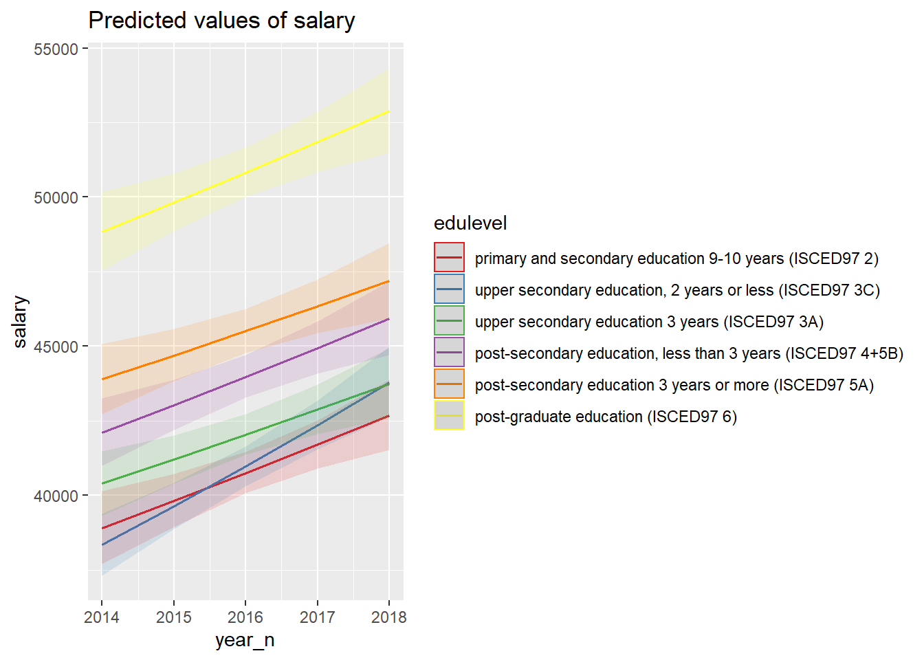
Figure 19: SSYK 214, Architects, engineers and related professionals, Year 2014 - 2018
plot(model, which = 1)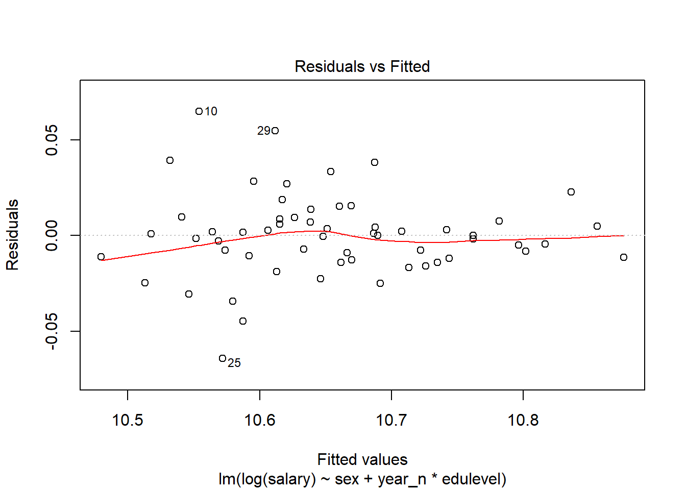
Figure 20: SSYK 214, Architects, engineers and related professionals, Year 2014 - 2018
tb[10,]## # A tibble: 1 x 8
## sector `occuptional (~ sex `level of educat~ year salary year_n edulevel
## <chr> <chr> <chr> <chr> <chr> <dbl> <dbl> <chr>
## 1 0 all ~ 214 Engineering~ women post-secondary e~ 2014 38800 2014 post-sec~tb[25,]## # A tibble: 1 x 8
## sector `occuptional (~ sex `level of educat~ year salary year_n edulevel
## <chr> <chr> <chr> <chr> <chr> <dbl> <dbl> <chr>
## 1 0 all ~ 214 Engineering~ women post-secondary e~ 2015 41200 2015 post-sec~tb[29,]## # A tibble: 1 x 8
## sector `occuptional (~ sex `level of educat~ year salary year_n edulevel
## <chr> <chr> <chr> <chr> <chr> <dbl> <dbl> <chr>
## 1 0 all ~ 214 Engineering~ men upper secondary ~ 2016 42100 2016 upper se~model <- lm(log(salary) ~ sex + year_n * bs(eduyears, knots = c(14)), data = tbnum)
summary(model) %>%
tidy() %>%
knitr::kable(
booktabs = TRUE,
caption = 'Summary from linear model fit')| term | estimate | std.error | statistic | p.value |
|---|---|---|---|---|
| (Intercept) | -37.5638852 | 12.5188542 | -3.0005849 | 0.0042648 |
| sexwomen | -0.0744192 | 0.0064006 | -11.6269343 | 0.0000000 |
| year_n | 0.0238981 | 0.0062092 | 3.8488437 | 0.0003504 |
| bs(eduyears, knots = c(14))1 | -33.5129947 | 34.8826450 | -0.9607355 | 0.3415000 |
| bs(eduyears, knots = c(14))2 | 52.9743796 | 67.5504892 | 0.7842190 | 0.4367647 |
| bs(eduyears, knots = c(14))3 | -26.1485331 | 82.0008933 | -0.3188811 | 0.7512002 |
| bs(eduyears, knots = c(14))4 | 8.2849059 | 16.6914080 | 0.4963575 | 0.6219077 |
| year_n:bs(eduyears, knots = c(14))1 | 0.0166181 | 0.0173024 | 0.9604499 | 0.3416422 |
| year_n:bs(eduyears, knots = c(14))2 | -0.0262412 | 0.0335071 | -0.7831529 | 0.4373844 |
| year_n:bs(eduyears, knots = c(14))3 | 0.0130625 | 0.0406748 | 0.3211439 | 0.7494955 |
| year_n:bs(eduyears, knots = c(14))4 | -0.0039997 | 0.0082789 | -0.4831182 | 0.6312082 |
summary(model)$adj.r.squared ## [1] 0.9302821Anova(model, type = 2)## Anova Table (Type II tests)
##
## Response: log(salary)
## Sum Sq Df F value Pr(>F)
## sex 0.08110 1 135.1856 1.453e-15 ***
## year_n 0.05941 1 99.0272 2.972e-13 ***
## bs(eduyears, knots = c(14)) 0.34299 4 142.9343 < 2.2e-16 ***
## year_n:bs(eduyears, knots = c(14)) 0.00179 4 0.7457 0.5657
## Residuals 0.02880 48
## ---
## Signif. codes: 0 '***' 0.001 '**' 0.01 '*' 0.05 '.' 0.1 ' ' 1plot_model(model, type = "pred", terms = c("year_n", "eduyears"))## Model has log-transformed response. Back-transforming predictions to original response scale. Standard errors are still on the log-scale.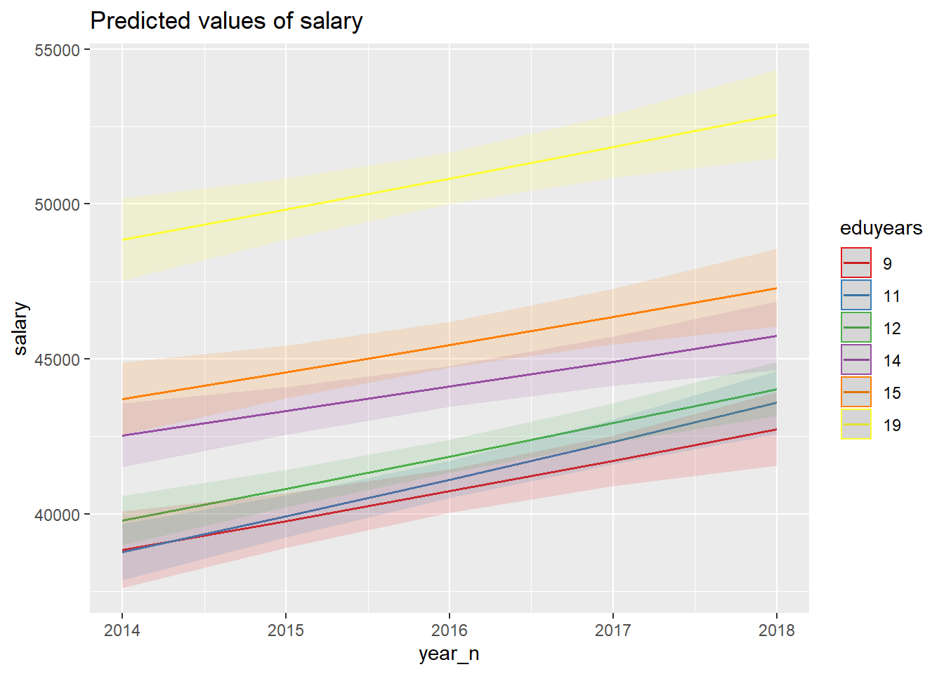
Figure 21: SSYK 214, Architects, engineers and related professionals, Year 2014 - 2018
plot(model, which = 1)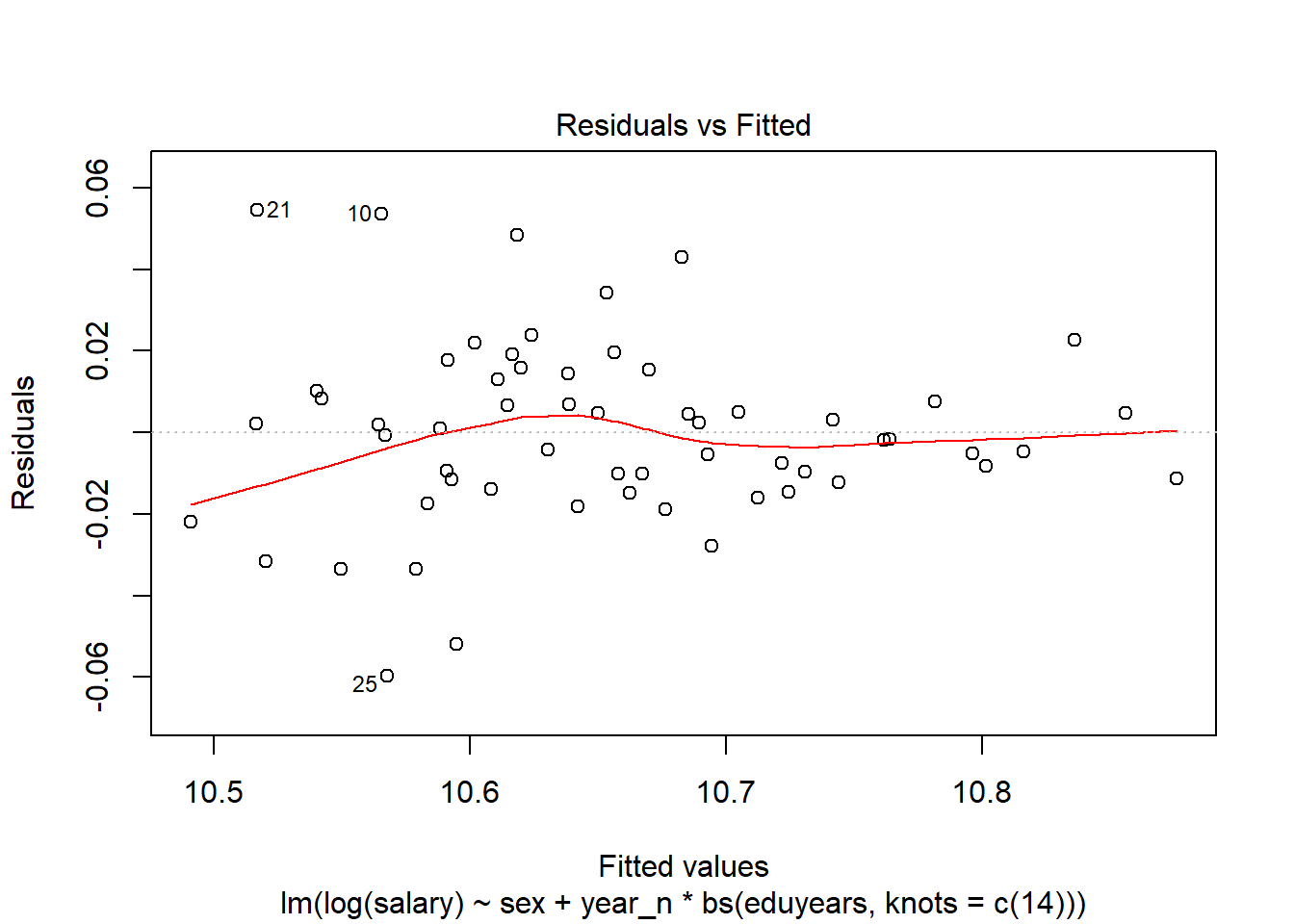
Figure 22: SSYK 214, Architects, engineers and related professionals, Year 2014 - 2018
tb[25,]## # A tibble: 1 x 8
## sector `occuptional (~ sex `level of educat~ year salary year_n edulevel
## <chr> <chr> <chr> <chr> <chr> <dbl> <dbl> <chr>
## 1 0 all ~ 214 Engineering~ women post-secondary e~ 2015 41200 2015 post-sec~Examine the interaction between gender and education. The only significant difference in salaries for the length in education is for the group upper secondary education, 2 years or less.
The F-value from the Anova table for the interaction term between gender and education is 3,3 (Pr(>F) < 0.01195), sufficient for rejecting the null hypothesis that the interaction between gender and education has no effect on the salary holding year as constant.
model <- lm(log(salary) ~ sex * edulevel + year_n, data = tbnum)

summary(model) %>%
  tidy() %>%
  knitr::kable(
  booktabs = TRUE,
caption = 'Summary from linear model fit')| term | estimate | std.error | statistic | p.value |
|---|---|---|---|---|
| (Intercept) | -34.7430460 | 4.1272331 | -8.4179994 | 0.0000000 |
| sexwomen | -0.0771083 | 0.0138850 | -5.5533508 | 0.0000013 |
| edulevelpost-secondary education 3 years or more (ISCED97 5A) | -0.1168022 | 0.0138850 | -8.4121058 | 0.0000000 |
| edulevelpost-secondary education, less than 3 years (ISCED97 4+5B) | -0.1597128 | 0.0138850 | -11.5025341 | 0.0000000 |
| edulevelprimary and secondary education 9-10 years (ISCED97 2) | -0.2251088 | 0.0138850 | -16.2123615 | 0.0000000 |
| edulevelupper secondary education 3 years (ISCED97 3A) | -0.1948942 | 0.0138850 | -14.0363072 | 0.0000000 |
| edulevelupper secondary education, 2 years or less (ISCED97 3C) | -0.1931089 | 0.0138850 | -13.9077238 | 0.0000000 |
| year_n | 0.0226094 | 0.0020472 | 11.0438961 | 0.0000000 |
| sexwomen:edulevelpost-secondary education 3 years or more (ISCED97 5A) | 0.0127331 | 0.0196364 | 0.6484450 | 0.5199213 |
| sexwomen:edulevelpost-secondary education, less than 3 years (ISCED97 4+5B) | 0.0301109 | 0.0196364 | 1.5334243 | 0.1320210 |
| sexwomen:edulevelprimary and secondary education 9-10 years (ISCED97 2) | 0.0094897 | 0.0202666 | 0.4682454 | 0.6418203 |
| sexwomen:edulevelupper secondary education 3 years (ISCED97 3A) | 0.0100153 | 0.0196364 | 0.5100385 | 0.6124632 |
| sexwomen:edulevelupper secondary education, 2 years or less (ISCED97 3C) | -0.0447952 | 0.0196364 | -2.2812368 | 0.0272117 |
summary(model)$adj.r.squared ## [1] 0.9439866Anova(model, type = 2)## Anova Table (Type II tests)
##
## Response: log(salary)
## Sum Sq Df F value Pr(>F)
## sex 0.08124 1 168.5530 < 2.2e-16 ***
## edulevel 0.34338 5 142.4863 < 2.2e-16 ***
## year_n 0.05879 1 121.9676 1.576e-14 ***
## sex:edulevel 0.00802 5 3.3293 0.01195 *
## Residuals 0.02217 46
## ---
## Signif. codes: 0 '***' 0.001 '**' 0.01 '*' 0.05 '.' 0.1 ' ' 1plot_model(model, type = "pred", terms = c("edulevel", "sex"))## Model has log-transformed response. Back-transforming predictions to original response scale. Standard errors are still on the log-scale.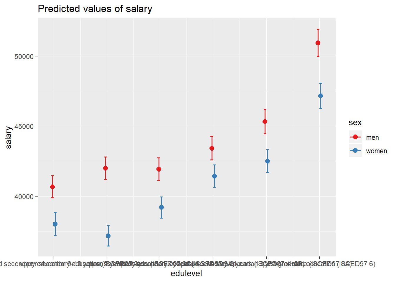
Figure 23: SSYK 214, Architects, engineers and related professionals, Year 2014 - 2018
plot(model, which = 1)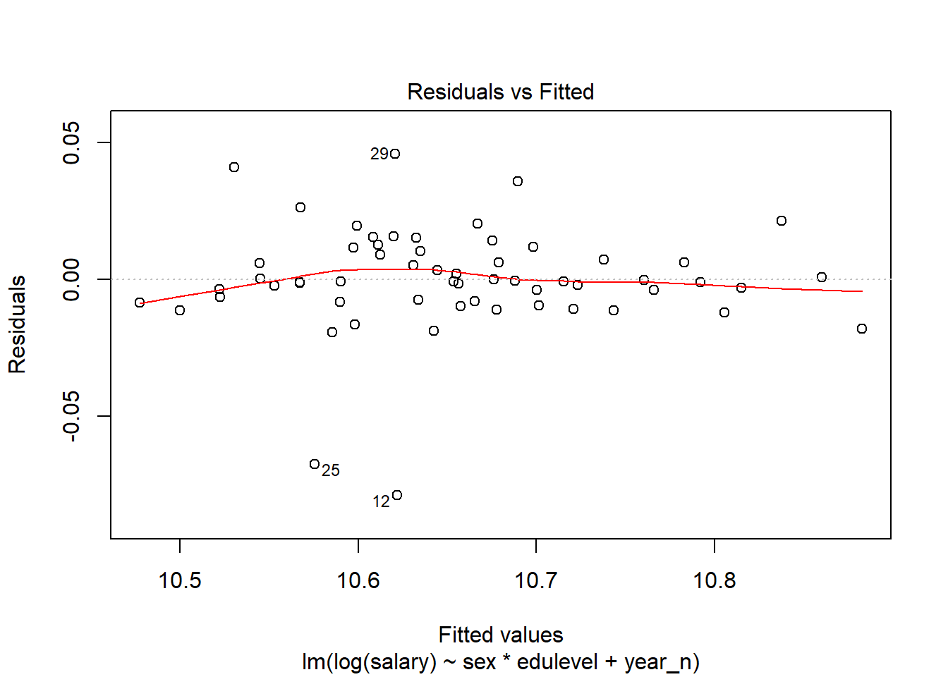
Figure 24: SSYK 214, Architects, engineers and related professionals, Year 2014 - 2018
tb[12,]## # A tibble: 1 x 8
## sector `occuptional (S~ sex `level of educa~ year salary year_n edulevel
## <chr> <chr> <chr> <chr> <chr> <dbl> <dbl> <chr>
## 1 0 all ~ 214 Engineering ~ women post-graduate e~ 2014 45000 2014 post-gra~model <- lm(log(salary) ~ sex * bs(eduyears, knots = c(14)) + year_n, data = tbnum)
summary(model) %>%
tidy() %>%
knitr::kable(
booktabs = TRUE,
caption = 'Summary from linear model fit')| term | estimate | std.error | statistic | p.value |
|---|---|---|---|---|
| (Intercept) | -35.0137987 | 4.1599657 | -8.4168479 | 0.0000000 |
| sexwomen | -0.0691630 | 0.0148436 | -4.6594632 | 0.0000254 |
| bs(eduyears, knots = c(14))1 | 0.0563505 | 0.0303035 | 1.8595384 | 0.0690857 |
| bs(eduyears, knots = c(14))2 | -0.0451702 | 0.0604863 | -0.7467842 | 0.4588363 |
| bs(eduyears, knots = c(14))3 | 0.2884546 | 0.0731010 | 3.9459725 | 0.0002585 |
| bs(eduyears, knots = c(14))4 | 0.2248785 | 0.0139796 | 16.0861324 | 0.0000000 |
| year_n | 0.0226322 | 0.0020635 | 10.9680236 | 0.0000000 |
| sexwomen:bs(eduyears, knots = c(14))1 | -0.1362989 | 0.0434669 | -3.1356935 | 0.0029251 |
| sexwomen:bs(eduyears, knots = c(14))2 | 0.2339328 | 0.0855779 | 2.7335654 | 0.0087471 |
| sexwomen:bs(eduyears, knots = c(14))3 | -0.2077223 | 0.1036306 | -2.0044483 | 0.0506812 |
| sexwomen:bs(eduyears, knots = c(14))4 | -0.0079140 | 0.0203999 | -0.3879451 | 0.6997718 |
summary(model)$adj.r.squared ## [1] 0.943092Anova(model, type = 2)## Anova Table (Type II tests)
##
## Response: log(salary)
## Sum Sq Df F value Pr(>F)
## sex 0.08128 1 165.9766 < 2.2e-16 ***
## bs(eduyears, knots = c(14)) 0.34299 4 175.1086 < 2.2e-16 ***
## year_n 0.05891 1 120.2975 1.128e-14 ***
## sex:bs(eduyears, knots = c(14)) 0.00708 4 3.6147 0.01181 *
## Residuals 0.02350 48
## ---
## Signif. codes: 0 '***' 0.001 '**' 0.01 '*' 0.05 '.' 0.1 ' ' 1plot_model(model, type = "pred", terms = c("eduyears", "sex"))## Model has log-transformed response. Back-transforming predictions to original response scale. Standard errors are still on the log-scale.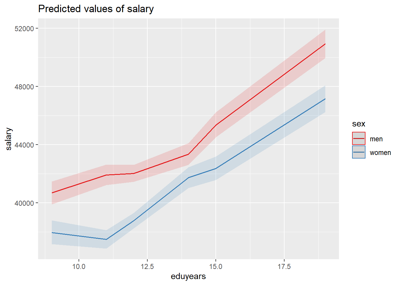
Figure 25: SSYK 214, Architects, engineers and related professionals, Year 2014 - 2018
plot(model, which = 1)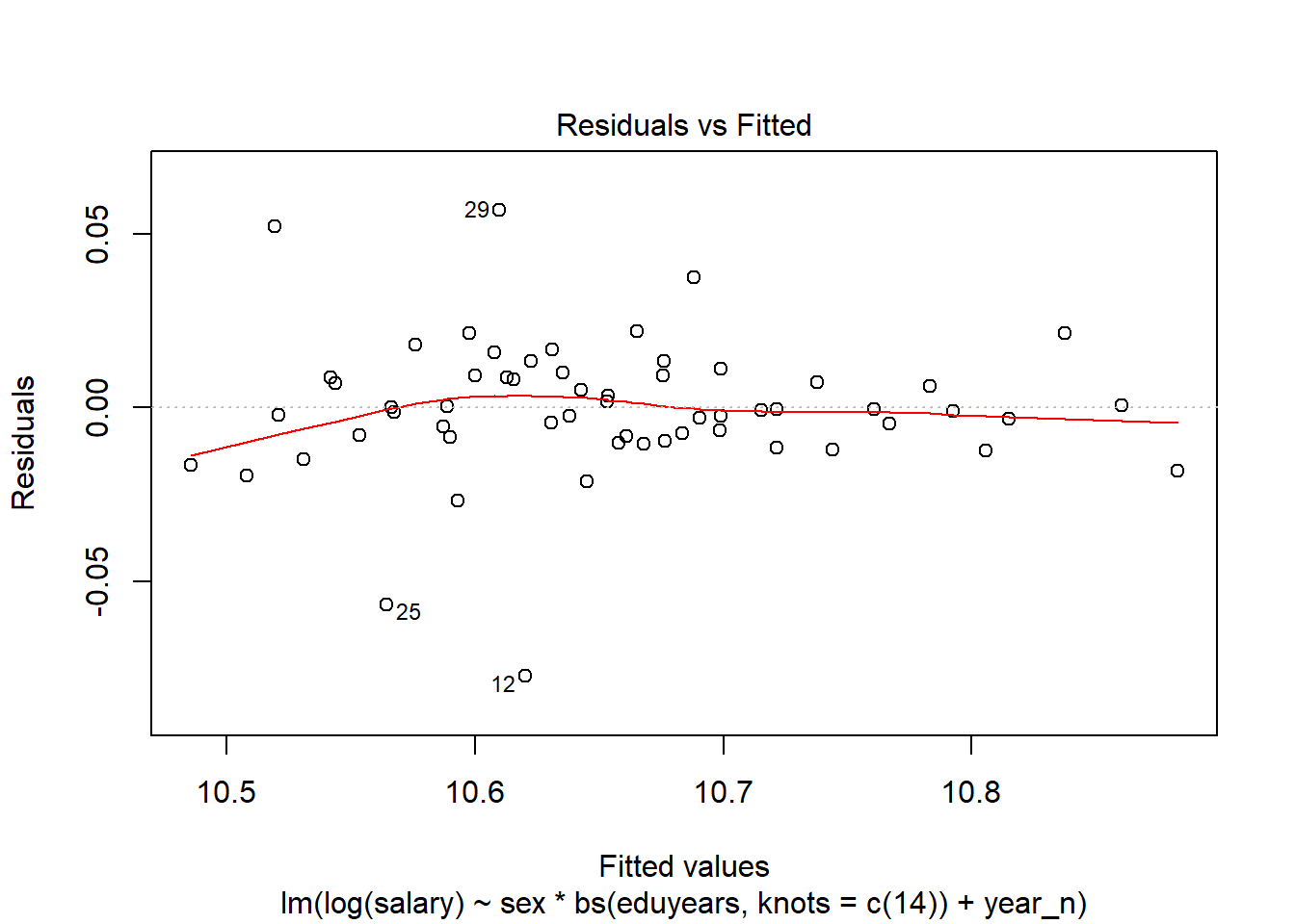
Figure 26: SSYK 214, Architects, engineers and related professionals, Year 2014 - 2018
Examine the interaction between gender and year There is no evidence that the salaries for men and women are interacting with year, holding education constant.
model <- lm(log(salary) ~ sex * year_n + edulevel, data = tbnum)

summary(model) %>%
  tidy() %>%
  knitr::kable(
  booktabs = TRUE,
caption = 'Summary from linear model fit')| term | estimate | std.error | statistic | p.value |
|---|---|---|---|---|
| (Intercept) | -33.2392045 | 6.3870956 | -5.2041188 | 0.0000037 |
| sexwomen | -3.4777309 | 9.2153884 | -0.3773830 | 0.7074862 |
| year_n | 0.0218628 | 0.0031682 | 6.9007009 | 0.0000000 |
| edulevelpost-secondary education 3 years or more (ISCED97 5A) | -0.1104356 | 0.0109750 | -10.0625026 | 0.0000000 |
| edulevelpost-secondary education, less than 3 years (ISCED97 4+5B) | -0.1446573 | 0.0109750 | -13.1806660 | 0.0000000 |
| edulevelprimary and secondary education 9-10 years (ISCED97 2) | -0.2209486 | 0.0113059 | -19.5427007 | 0.0000000 |
| edulevelupper secondary education 3 years (ISCED97 3A) | -0.1898866 | 0.0109750 | -17.3017955 | 0.0000000 |
| edulevelupper secondary education, 2 years or less (ISCED97 3C) | -0.2155065 | 0.0109750 | -19.6361878 | 0.0000000 |
| sexwomen:year_n | 0.0016882 | 0.0045710 | 0.3693193 | 0.7134493 |
summary(model)$adj.r.squared ## [1] 0.93001Anova(model, type = 2)## Anova Table (Type II tests)
##
## Response: log(salary)
## Sum Sq Df F value Pr(>F)
## sex 0.08124 1 134.8940 8.258e-16 ***
## year_n 0.05936 1 98.5705 2.047e-13 ***
## edulevel 0.34343 5 114.0493 < 2.2e-16 ***
## sex:year_n 0.00008 1 0.1364 0.7134
## Residuals 0.03011 50
## ---
## Signif. codes: 0 '***' 0.001 '**' 0.01 '*' 0.05 '.' 0.1 ' ' 1plot_model(model, type = "pred", terms = c("year_n", "sex"))## Model has log-transformed response. Back-transforming predictions to original response scale. Standard errors are still on the log-scale.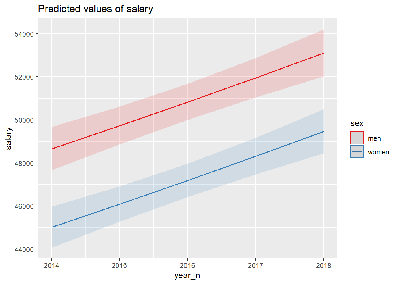
Figure 27: SSYK 214, Architects, engineers and related professionals, Year 2014 - 2018
plot(model, which = 1)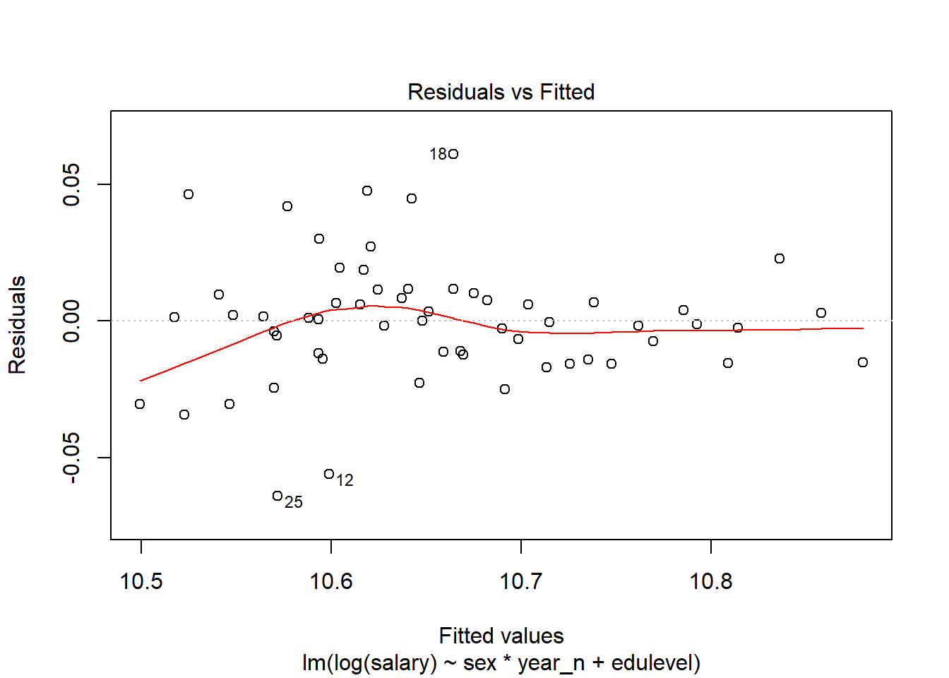
Figure 28: SSYK 214, Architects, engineers and related professionals, Year 2014 - 2018
tb[18,]## # A tibble: 1 x 8
## sector `occuptional (~ sex `level of educat~ year salary year_n edulevel
## <chr> <chr> <chr> <chr> <chr> <dbl> <dbl> <chr>
## 1 0 all ~ 214 Engineering~ men post-secondary e~ 2015 44800 2015 post-sec~model <- lm(log(salary) ~ sex * year_n + bs(eduyears, knots = c(14)), data = tbnum)
summary(model) %>%
tidy() %>%
knitr::kable(
booktabs = TRUE,
caption = 'Summary from linear model fit')| term | estimate | std.error | statistic | p.value |
|---|---|---|---|---|
| (Intercept) | -33.4606036 | 6.3648511 | -5.2570914 | 0.0000029 |
| sexwomen | -3.5113836 | 9.1831982 | -0.3823704 | 0.7037755 |
| year_n | 0.0218628 | 0.0031572 | 6.9248186 | 0.0000000 |
| bs(eduyears, knots = c(14))1 | -0.0110825 | 0.0239981 | -0.4618072 | 0.6461835 |
| bs(eduyears, knots = c(14))2 | 0.0720456 | 0.0472864 | 1.5236020 | 0.1337855 |
| bs(eduyears, knots = c(14))3 | 0.1853033 | 0.0572546 | 3.2364779 | 0.0021284 |
| bs(eduyears, knots = c(14))4 | 0.2214175 | 0.0112515 | 19.6788574 | 0.0000000 |
| sexwomen:year_n | 0.0017049 | 0.0045551 | 0.3742767 | 0.7097502 |
summary(model)$adj.r.squared ## [1] 0.9304967Anova(model, type = 2)## Anova Table (Type II tests)
##
## Response: log(salary)
## Sum Sq Df F value Pr(>F)
## sex 0.08128 1 135.8986 5.361e-16 ***
## year_n 0.05941 1 99.3330 1.446e-13 ***
## bs(eduyears, knots = c(14)) 0.34304 4 143.3973 < 2.2e-16 ***
## sex:year_n 0.00008 1 0.1401 0.7098
## Residuals 0.03050 51
## ---
## Signif. codes: 0 '***' 0.001 '**' 0.01 '*' 0.05 '.' 0.1 ' ' 1plot_model(model, type = "pred", terms = c("eduyears", "sex"))## Model has log-transformed response. Back-transforming predictions to original response scale. Standard errors are still on the log-scale.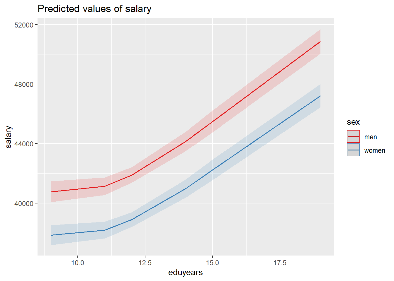
Figure 29: SSYK 214, Architects, engineers and related professionals, Year 2014 - 2018
plot(model, which = 1)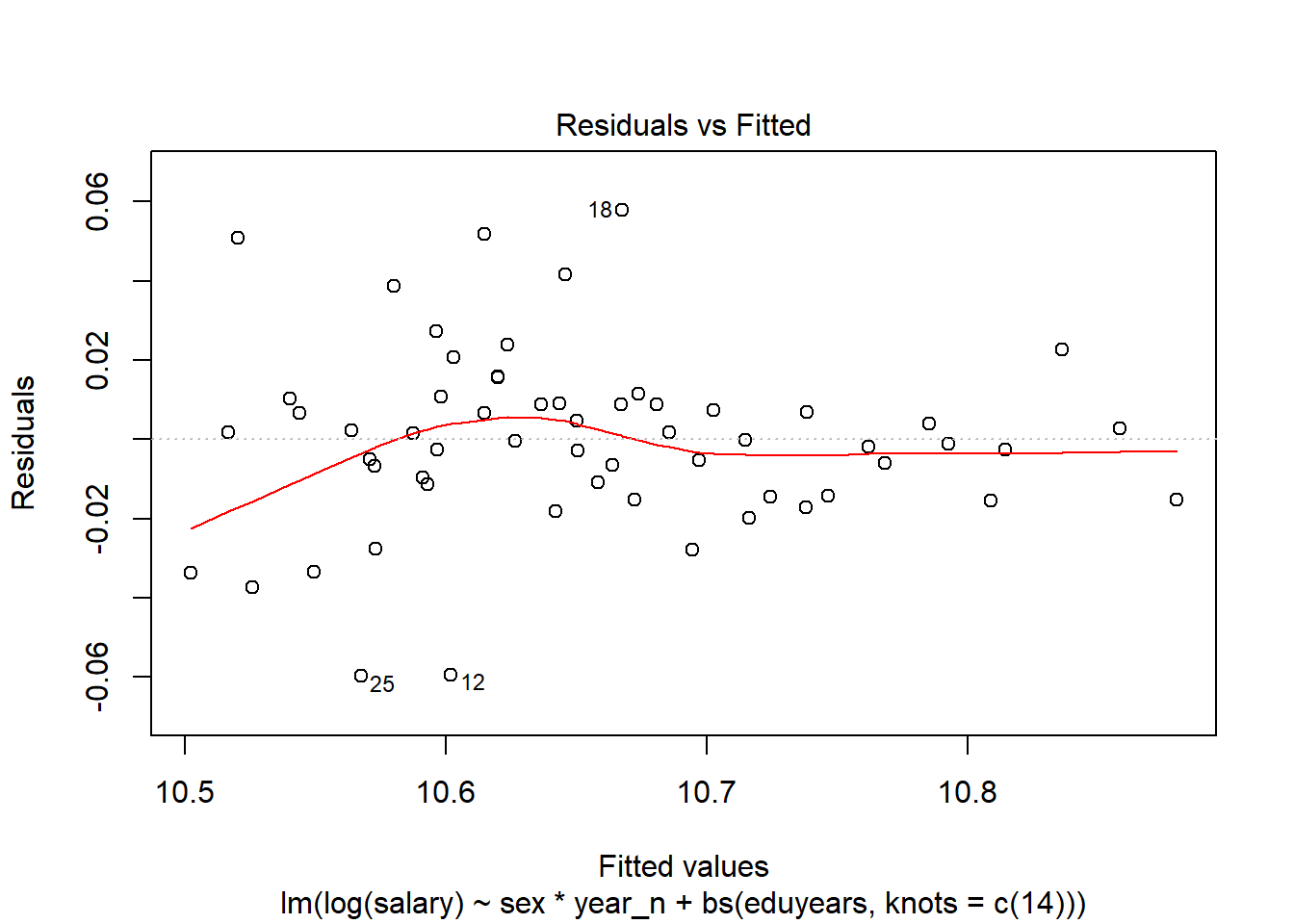
Figure 30: SSYK 214, Architects, engineers and related professionals, Year 2014 - 2018
Examine the interaction between year, gender and education It’s becoming a bit difficult to make any significant predictions from the model, the data is not sufficiently large, the degrees of freedom has been reduced from 51 in the model with no interaction terms to 35.
There are no significant interaction terms in the summary.
The F-value from the Anova table for the interaction term between gender and education is 3,0 (Pr(>F) < 0.02377), sufficient for rejecting the null hypothesis that the interaction between gender and education has no effect on the salary holding year as constant.
model <- lm(log(salary) ~ sex * year_n * edulevel, data = tbnum)

summary(model) %>%
  tidy() %>%
  knitr::kable(
  booktabs = TRUE,
caption = 'Summary from linear model fit')| term | estimate | std.error | statistic | p.value |
|---|---|---|---|---|
| (Intercept) | -28.6598716 | 14.7502103 | -1.9430144 | 0.0600924 |
| sexwomen | -1.3628373 | 20.8599474 | -0.0653327 | 0.9482808 |
| year_n | 0.0195920 | 0.0073166 | 2.6777544 | 0.0112090 |
| edulevelpost-secondary education 3 years or more (ISCED97 5A) | 5.7063531 | 20.8599474 | 0.2735555 | 0.7860341 |
| edulevelpost-secondary education, less than 3 years (ISCED97 4+5B) | 1.8926757 | 20.8599474 | 0.0907325 | 0.9282224 |
| edulevelprimary and secondary education 9-10 years (ISCED97 2) | -6.5228901 | 20.8599474 | -0.3126993 | 0.7563648 |
| edulevelupper secondary education 3 years (ISCED97 3A) | 3.4041093 | 20.8599474 | 0.1631888 | 0.8713084 |
| edulevelupper secondary education, 2 years or less (ISCED97 3C) | -32.8376799 | 20.8599474 | -1.5741976 | 0.1244390 |
| sexwomen:year_n | 0.0006378 | 0.0103472 | 0.0616363 | 0.9512031 |
| sexwomen:edulevelpost-secondary education 3 years or more (ISCED97 5A) | -4.3942731 | 29.5004205 | -0.1489563 | 0.8824431 |
| sexwomen:edulevelpost-secondary education, less than 3 years (ISCED97 4+5B) | -11.2850561 | 29.5004205 | -0.3825388 | 0.7043750 |
| sexwomen:edulevelprimary and secondary education 9-10 years (ISCED97 2) | 1.3504648 | 32.9857439 | 0.0409409 | 0.9675757 |
| sexwomen:edulevelupper secondary education 3 years (ISCED97 3A) | -7.4704416 | 29.5004205 | -0.2532317 | 0.8015707 |
| sexwomen:edulevelupper secondary education, 2 years or less (ISCED97 3C) | 11.3890513 | 29.5004205 | 0.3860640 | 0.7017862 |
| year_n:edulevelpost-secondary education 3 years or more (ISCED97 5A) | -0.0028885 | 0.0103472 | -0.2791549 | 0.7817689 |
| year_n:edulevelpost-secondary education, less than 3 years (ISCED97 4+5B) | -0.0010180 | 0.0103472 | -0.0983890 | 0.9221848 |
| year_n:edulevelprimary and secondary education 9-10 years (ISCED97 2) | 0.0031239 | 0.0103472 | 0.3019079 | 0.7645090 |
| year_n:edulevelupper secondary education 3 years (ISCED97 3A) | -0.0017852 | 0.0103472 | -0.1725318 | 0.8640133 |
| year_n:edulevelupper secondary education, 2 years or less (ISCED97 3C) | 0.0161927 | 0.0103472 | 1.5649406 | 0.1265947 |
| sexwomen:year_n:edulevelpost-secondary education 3 years or more (ISCED97 5A) | 0.0021860 | 0.0146331 | 0.1493879 | 0.8821050 |
| sexwomen:year_n:edulevelpost-secondary education, less than 3 years (ISCED97 4+5B) | 0.0056127 | 0.0146331 | 0.3835596 | 0.7036250 |
| sexwomen:year_n:edulevelprimary and secondary education 9-10 years (ISCED97 2) | -0.0006652 | 0.0163603 | -0.0406584 | 0.9677993 |
| sexwomen:year_n:edulevelupper secondary education 3 years (ISCED97 3A) | 0.0037105 | 0.0146331 | 0.2535713 | 0.8013105 |
| sexwomen:year_n:edulevelupper secondary education, 2 years or less (ISCED97 3C) | -0.0056716 | 0.0146331 | -0.3875826 | 0.7006721 |
summary(model)$adj.r.squared ## [1] 0.9377879Anova(model, type = 2)## Anova Table (Type II tests)
##
## Response: log(salary)
## Sum Sq Df F value Pr(>F)
## sex 0.08897 6 27.6985 6.428e-12 ***
## year_n 0.05879 1 109.8150 2.456e-12 ***
## edulevel 0.35144 10 65.6498 < 2.2e-16 ***
## sex:year_n 0.00007 1 0.1338 0.71677
## sex:edulevel 0.00800 5 2.9902 0.02377 *
## year_n:edulevel 0.00298 5 1.1127 0.37150
## sex:year_n:edulevel 0.00039 5 0.1445 0.98038
## Residuals 0.01874 35
## ---
## Signif. codes: 0 '***' 0.001 '**' 0.01 '*' 0.05 '.' 0.1 ' ' 1plot_model(model, type = "pred", terms = c("year_n", "edulevel","sex"))## Model has log-transformed response. Back-transforming predictions to original response scale. Standard errors are still on the log-scale.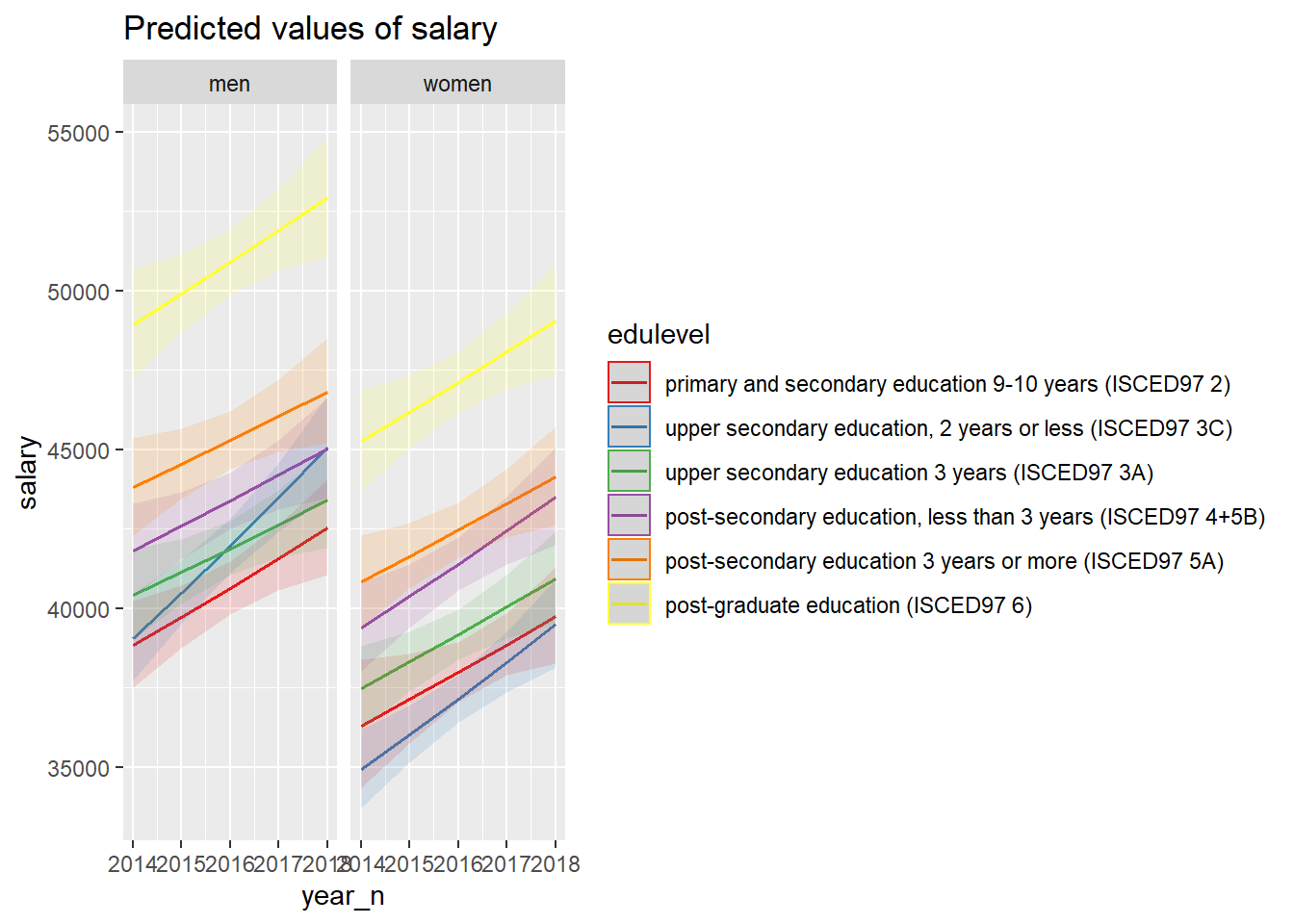
Figure 31: SSYK 214, Architects, engineers and related professionals, Year 2014 - 2018
plot(model, which = 1)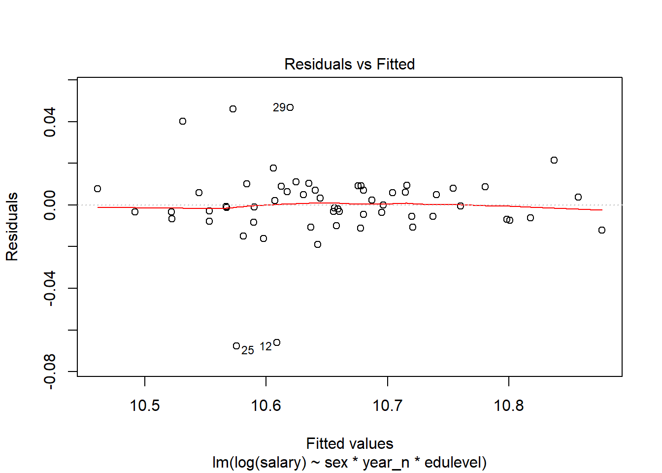
Figure 32: SSYK 214, Architects, engineers and related professionals, Year 2014 - 2018
tb[29,]## # A tibble: 1 x 8
## sector `occuptional (~ sex `level of educat~ year salary year_n edulevel
## <chr> <chr> <chr> <chr> <chr> <dbl> <dbl> <chr>
## 1 0 all ~ 214 Engineering~ men upper secondary ~ 2016 42100 2016 upper se~model <- lm(log(salary) ~ sex * year_n * bs(eduyears, knots = c(14)), data = tbnum)
summary(model) %>%
tidy() %>%
knitr::kable(
booktabs = TRUE,
caption = 'Summary from linear model fit')| term | estimate | std.error | statistic | p.value |
|---|---|---|---|---|
| (Intercept) | -36.4297072 | 14.8747312 | -2.4491002 | 0.0189181 |
| sexwomen | -1.4146024 | 25.7220917 | -0.0549956 | 0.9564227 |
| year_n | 0.0233345 | 0.0073783 | 3.1625710 | 0.0030250 |
| bs(eduyears, knots = c(14))1 | -52.0255138 | 45.6462798 | -1.1397536 | 0.2613408 |
| bs(eduyears, knots = c(14))2 | 93.3207084 | 91.1108278 | 1.0242549 | 0.3120264 |
| bs(eduyears, knots = c(14))3 | -61.4602190 | 110.1124840 | -0.5581585 | 0.5799266 |
| bs(eduyears, knots = c(14))4 | 7.8004982 | 21.0576228 | 0.3704358 | 0.7130621 |
| sexwomen:year_n | 0.0006670 | 0.0127569 | 0.0522889 | 0.9585654 |
| sexwomen:bs(eduyears, knots = c(14))1 | 35.6845382 | 68.0014005 | 0.5247618 | 0.6027192 |
| sexwomen:bs(eduyears, knots = c(14))2 | -81.1592876 | 129.0648894 | -0.6288255 | 0.5331293 |
| sexwomen:bs(eduyears, knots = c(14))3 | 69.2953946 | 157.1561131 | 0.4409335 | 0.6616959 |
| sexwomen:bs(eduyears, knots = c(14))4 | 0.0407412 | 33.2552425 | 0.0012251 | 0.9990288 |
| year_n:bs(eduyears, knots = c(14))1 | 0.0258343 | 0.0226420 | 1.1409884 | 0.2608328 |
| year_n:bs(eduyears, knots = c(14))2 | -0.0463124 | 0.0451939 | -1.0247509 | 0.3117952 |
| year_n:bs(eduyears, knots = c(14))3 | 0.0306293 | 0.0546193 | 0.5607783 | 0.5781565 |
| year_n:bs(eduyears, knots = c(14))4 | -0.0037577 | 0.0104452 | -0.3597567 | 0.7209699 |
| sexwomen:year_n:bs(eduyears, knots = c(14))1 | -0.0177678 | 0.0337292 | -0.5267776 | 0.6013316 |
| sexwomen:year_n:bs(eduyears, knots = c(14))2 | 0.0403738 | 0.0640202 | 0.6306418 | 0.5319531 |
| sexwomen:year_n:bs(eduyears, knots = c(14))3 | -0.0344753 | 0.0779537 | -0.4422531 | 0.6607490 |
| sexwomen:year_n:bs(eduyears, knots = c(14))4 | -0.0000238 | 0.0164940 | -0.0014428 | 0.9988562 |
summary(model)$adj.r.squared ## [1] 0.9364598Anova(model, type = 2)## Anova Table (Type II tests)
##
## Response: log(salary)
## Sum Sq Df F value Pr(>F)
## sex 0.08817 5 32.2521 7.295e-13 ***
## year_n 0.05891 1 107.7412 8.809e-13 ***
## bs(eduyears, knots = c(14)) 0.35011 8 80.0434 < 2.2e-16 ***
## sex:year_n 0.00008 1 0.1517 0.69908
## sex:bs(eduyears, knots = c(14)) 0.00706 4 3.2268 0.02218 *
## year_n:bs(eduyears, knots = c(14)) 0.00179 4 0.8168 0.52231
## sex:year_n:bs(eduyears, knots = c(14)) 0.00032 4 0.1468 0.96335
## Residuals 0.02132 39
## ---
## Signif. codes: 0 '***' 0.001 '**' 0.01 '*' 0.05 '.' 0.1 ' ' 1plot_model(model, type = "pred", terms = c("eduyears", "year_n","sex"))## Model has log-transformed response. Back-transforming predictions to original response scale. Standard errors are still on the log-scale.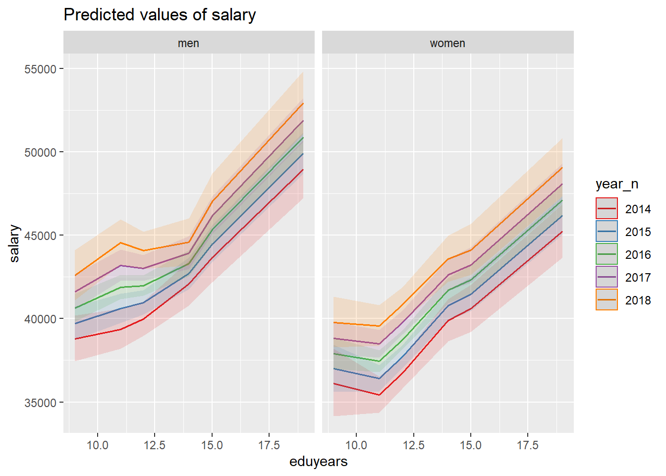
Figure 33: SSYK 214, Architects, engineers and related professionals, Year 2014 - 2018
plot(model, which = 1)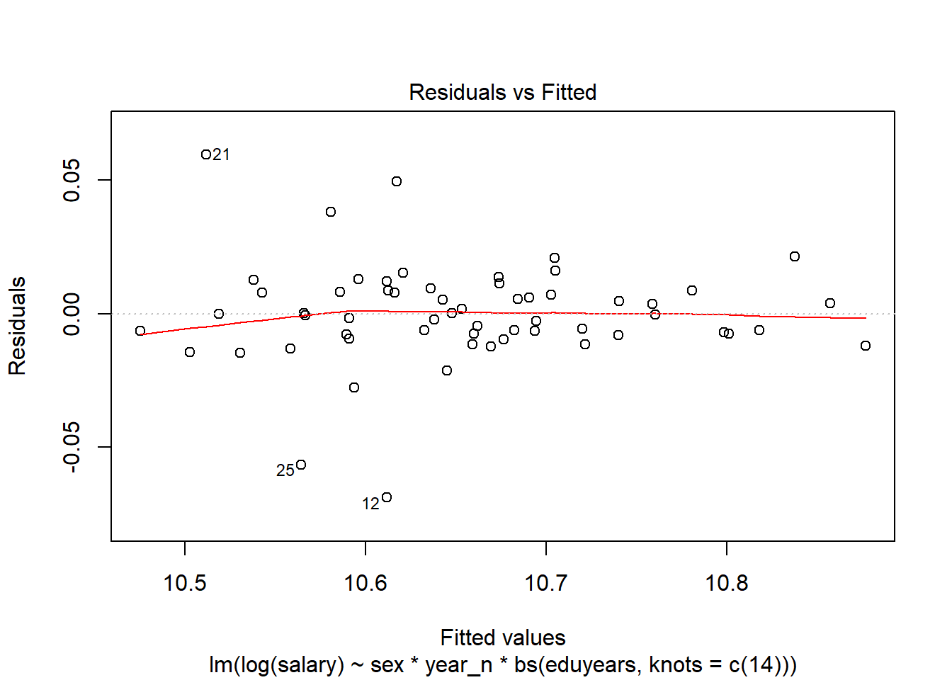
Figure 34: SSYK 214, Architects, engineers and related professionals, Year 2014 - 2018