So far I have analysed the effect of experience, education, gender and year on the salary of engineers in Sweden. In this post, I will have a look at the effect of the region on the salary of engineers in Sweden.
Statistics Sweden use NUTS (Nomenclature des Unités Territoriales Statistiques), which is the EU’s hierarchical regional division, to specify the regions.
First, define libraries and functions.
library (tidyverse) ## -- Attaching packages --------------------- tidyverse 1.3.0 --## v ggplot2 3.2.1 v purrr 0.3.3
## v tibble 2.1.3 v dplyr 0.8.3
## v tidyr 1.0.2 v stringr 1.4.0
## v readr 1.3.1 v forcats 0.4.0## -- Conflicts ------------------------ tidyverse_conflicts() --
## x dplyr::filter() masks stats::filter()
## x dplyr::lag() masks stats::lag()library (broom)
library (car)## Loading required package: carData##
## Attaching package: 'car'## The following object is masked from 'package:dplyr':
##
## recode## The following object is masked from 'package:purrr':
##
## somelibrary (swemaps) # devtools::install_github('reinholdsson/swemaps')
library(sjPlot)## Registered S3 methods overwritten by 'lme4':
## method from
## cooks.distance.influence.merMod car
## influence.merMod car
## dfbeta.influence.merMod car
## dfbetas.influence.merMod car## Install package "strengejacke" from GitHub (`devtools::install_github("strengejacke/strengejacke")`) to load all sj-packages at once!readfile <- function (file1){
read_csv (file1, col_types = cols(), locale = readr::locale (encoding = "latin1"), na = c("..", "NA")) %>%
gather (starts_with("19"), starts_with("20"), key = "year", value = salary) %>%
drop_na() %>%
mutate (year_n = parse_number (year))
}
nuts <- read.csv("nuts.csv") %>%
mutate(NUTS2_sh = substr(NUTS2, 1, 4))
map_ln_n <- map_ln %>%
mutate(lnkod_n = as.numeric(lnkod)) The data table is downloaded from Statistics Sweden. It is saved as a comma-delimited file without heading, 000000CG.csv, http://www.statistikdatabasen.scb.se/pxweb/en/ssd/.
The table: Average basic salary, monthly salary and women´s salary as a percentage of men´s salary by region, sector, occupational group (SSYK 2012) and sex. Year 2014 - 2018 Monthly salary All sectors
We expect that the region is an important factor in salaries. As a null hypothesis, we assume that the region is not related to the salary and examine if we can reject this hypothesis with the data from Statistics Sweden.
tb <- readfile ("000000CG.csv") %>%
  filter (`occuptional  (SSYK 2012)` == "214 Engineering professionals") %>%
  left_join(nuts %>% distinct (NUTS2_en, NUTS2_sh), by = c("region" = "NUTS2_en"))
## Warning: Column `region`/`NUTS2_en` joining character vector and factor,
## coercing into character vectortb_map <- readfile ("000000CG.csv") %>%
filter (`occuptional (SSYK 2012)` == "214 Engineering professionals") %>%
left_join(nuts, by = c("region" = "NUTS2_en")) ## Warning: Column `region`/`NUTS2_en` joining character vector and factor,
## coercing into character vectortb_map %>%
filter (sex == "men") %>%
right_join(map_ln_n, by = c("Länskod" = "lnkod_n")) %>%
ggplot() +
geom_polygon(mapping = aes(x = ggplot_long, y = ggplot_lat, group = lnkod, fill = salary)) +
facet_grid(. ~ year) +
coord_equal() 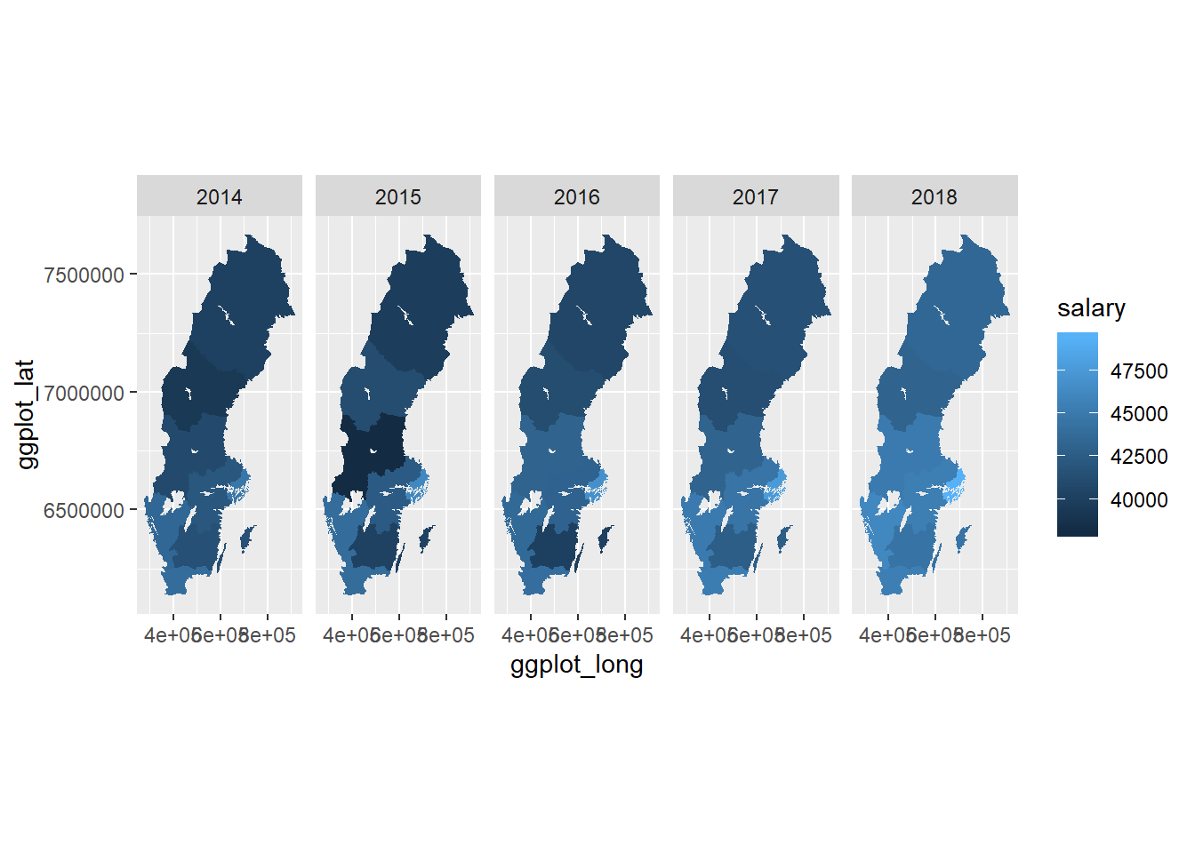
Figure 1: SSYK 214, Architects, engineers and related professionals, men, Year 2014 - 2018
tb_map %>%
  filter (sex == "women") %>%
  right_join(map_ln_n, by = c("Länskod" = "lnkod_n")) %>%
  ggplot() +
    geom_polygon(mapping = aes(x = ggplot_long, y = ggplot_lat, group = lnkod, fill = salary)) +
      facet_grid(. ~ year) +
coord_equal() 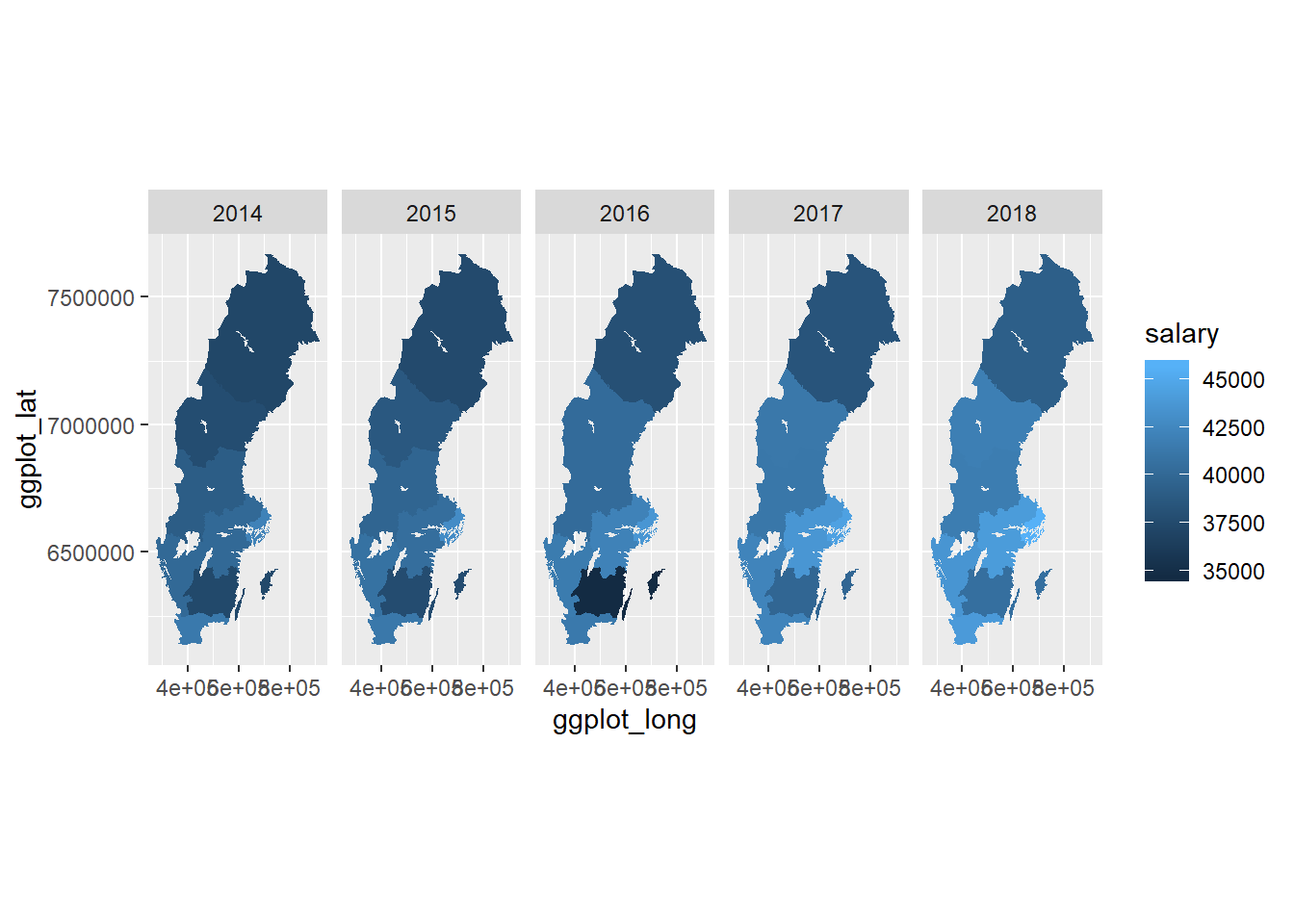
Figure 2: SSYK 214, Architects, engineers and related professionals, women, Year 2014 - 2018
tb %>%
  ggplot () +
    geom_point (mapping = aes(x = year_n, y = salary, colour = region, shape=sex)) +
  labs(
    x = "Year",
    y = "Salary (SEK/month)"
  )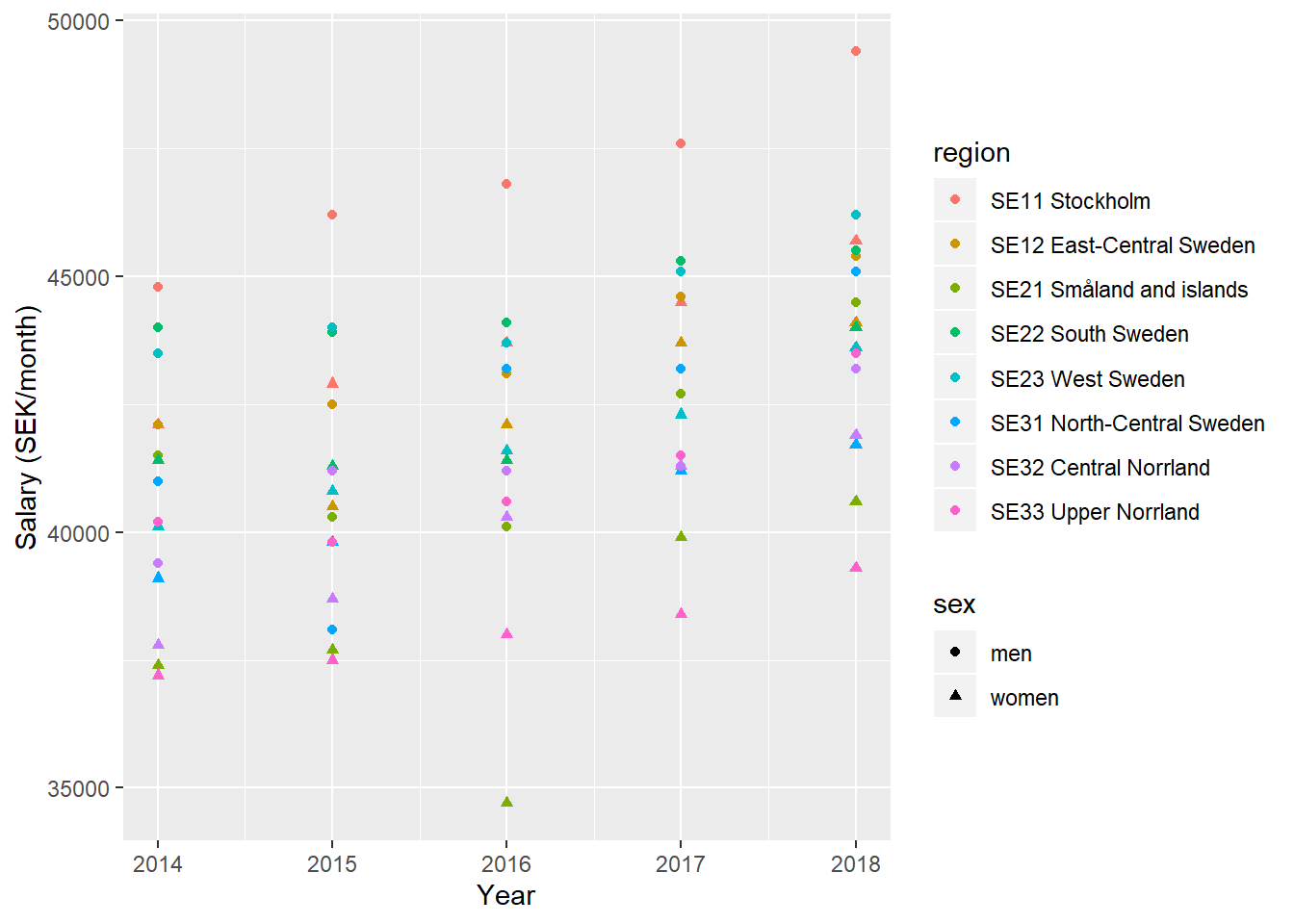
Figure 3: SSYK 214, Architects, engineers and related professionals, Year 2014 - 2018
The F-value from the Anova table for the region is 40 (Pr(>F) < 2.2e-16), sufficient for rejecting the null hypothesis that the region has no effect on the salary holding year as constant. The adjusted R-squared value is 0,882 implying a good fit of the model.
model <-lm (log(salary) ~ year_n + sex + region , data = tb)

tb <- bind_cols(tb, as_tibble(exp(predict(model, tb, interval = "confidence"))))

tb %>%
  ggplot () +
    geom_point (mapping = aes(x = year_n,y = fit, colour = region, shape=sex)) +
  labs(
    x = "Year",
    y = "Salary (SEK/month)"
  )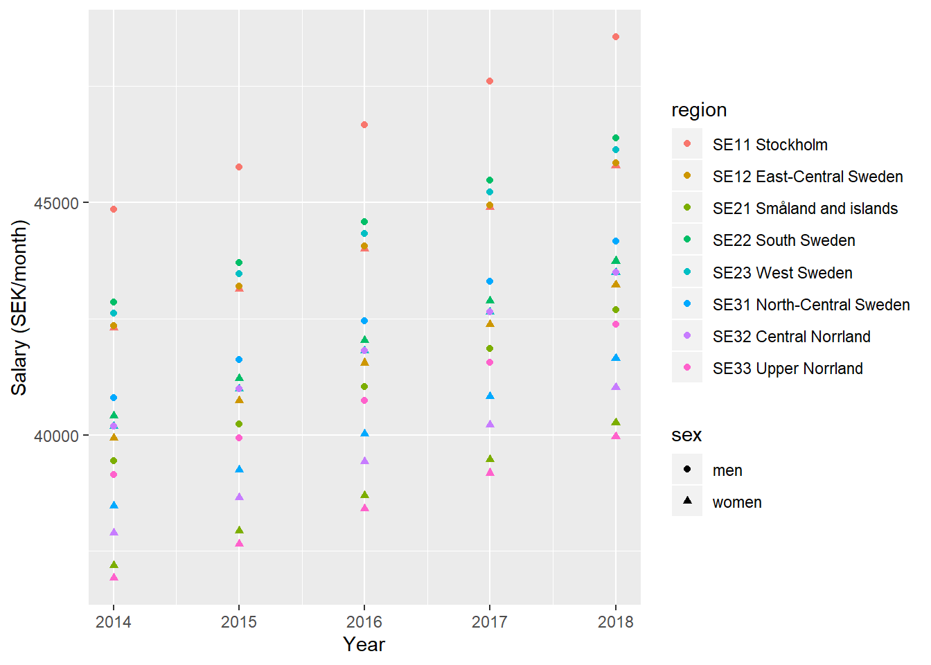
Figure 4: Model fit, SSYK 214, Architects, engineers and related professionals, Year 2014 - 2018
summary(model) %>%
  tidy() %>%
  knitr::kable(
  booktabs = TRUE,
caption = 'Summary from linear model fit')| term | estimate | std.error | statistic | p.value |
|---|---|---|---|---|
| (Intercept) | -29.2269335 | 3.7348614 | -7.825440 | 0.00e+00 |
| year_n | 0.0198303 | 0.0018526 | 10.703985 | 0.00e+00 |
| sexwomen | -0.0587056 | 0.0052400 | -11.203449 | 0.00e+00 |
| regionSE12 East-Central Sweden | -0.0574855 | 0.0104799 | -5.485297 | 6.00e-07 |
| regionSE21 Småland and islands | -0.1286385 | 0.0104799 | -12.274762 | 0.00e+00 |
| regionSE22 South Sweden | -0.0457725 | 0.0104799 | -4.367642 | 4.26e-05 |
| regionSE23 West Sweden | -0.0513546 | 0.0104799 | -4.900285 | 6.00e-06 |
| regionSE31 North-Central Sweden | -0.0948080 | 0.0104799 | -9.046630 | 0.00e+00 |
| regionSE32 Central Norrland | -0.1099716 | 0.0104799 | -10.493550 | 0.00e+00 |
| regionSE33 Upper Norrland | -0.1360235 | 0.0104799 | -12.979443 | 0.00e+00 |
summary(model)$r.squared## [1] 0.8817871Anova(model, type=2) %>%
tidy() %>%
knitr::kable(
booktabs = TRUE,
caption = 'Anova report from linear model fit')| term | sumsq | df | statistic | p.value |
|---|---|---|---|---|
| year_n | 0.0629183 | 1 | 114.57530 | 0 |
| sex | 0.0689270 | 1 | 125.51728 | 0 |
| region | 0.1548911 | 7 | 40.29419 | 0 |
| Residuals | 0.0384401 | 70 | NA | NA |
Let’s check what we have found.
model <-lm (log(salary) ~ year_n + sex + NUTS2_sh , data = tb)

plot_model(model, type = "pred", terms = c("NUTS2_sh"))
## Model has log-transformed response. Back-transforming predictions to original response scale. Standard errors are still on the log-scale.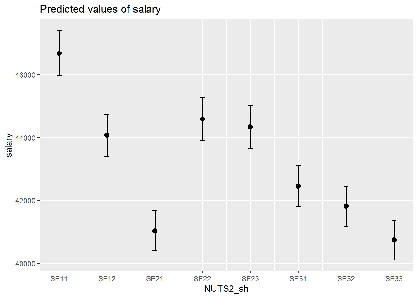
Figure 5: SSYK 214, Architects, engineers and related professionals, Year 2014 - 2018
plot(model, which = 1)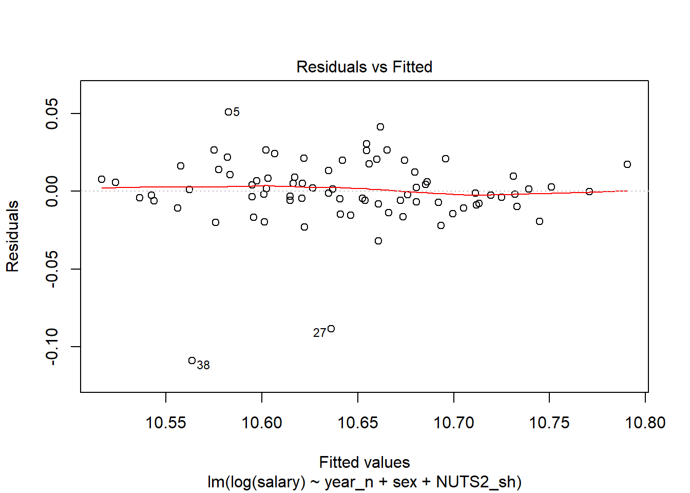
Figure 6: SSYK 214, Architects, engineers and related professionals, Year 2014 - 2018
tb[38,]## # A tibble: 1 x 11
## region sector `occuptional (~ sex year salary year_n NUTS2_sh fit
## <chr> <chr> <chr> <chr> <chr> <dbl> <dbl> <chr> <dbl>
## 1 SE21 ~ 0 all~ 214 Engineering~ women 2016 34700 2016 SE21 38698.
## # ... with 2 more variables: lwr <dbl>, upr <dbl>tb[27,]## # A tibble: 1 x 11
## region sector `occuptional (~ sex year salary year_n NUTS2_sh fit
## <chr> <chr> <chr> <chr> <chr> <dbl> <dbl> <chr> <dbl>
## 1 SE31 ~ 0 all~ 214 Engineering~ men 2015 38100 2015 SE31 41616.
## # ... with 2 more variables: lwr <dbl>, upr <dbl>tb[5,]## # A tibble: 1 x 11
## region sector `occuptional (~ sex year salary year_n NUTS2_sh fit
## <chr> <chr> <chr> <chr> <chr> <dbl> <dbl> <chr> <dbl>
## 1 SE21 ~ 0 all~ 214 Engineering~ men 2014 41500 2014 SE21 39442.
## # ... with 2 more variables: lwr <dbl>, upr <dbl>Also examine the interaction between gender and region. The F-value from the Anova table for the interaction is 2,7 (Pr(>F) < 0.017) implying a relation to 95 % significance.
model <-lm (log(salary) ~ year_n + sex * NUTS2_sh , data = tb)

summary(model) %>%
  tidy() %>%
  knitr::kable(
  booktabs = TRUE,
caption = 'Summary from linear model fit')| term | estimate | std.error | statistic | p.value |
|---|---|---|---|---|
| (Intercept) | -29.2212864 | 3.4559410 | -8.4553776 | 0.0000000 |
| year_n | 0.0198303 | 0.0017142 | 11.5678970 | 0.0000000 |
| sexwomen | -0.0699998 | 0.0137140 | -5.1042618 | 0.0000033 |
| NUTS2_shSE12 | -0.0755067 | 0.0137140 | -5.5058132 | 0.0000007 |
| NUTS2_shSE21 | -0.1161490 | 0.0137140 | -8.4693756 | 0.0000000 |
| NUTS2_shSE22 | -0.0520542 | 0.0137140 | -3.7957018 | 0.0003332 |
| NUTS2_shSE23 | -0.0535387 | 0.0137140 | -3.9039471 | 0.0002331 |
| NUTS2_shSE31 | -0.1099009 | 0.0137140 | -8.0137791 | 0.0000000 |
| NUTS2_shSE32 | -0.1293018 | 0.0137140 | -9.4284543 | 0.0000000 |
| NUTS2_shSE33 | -0.1327796 | 0.0137140 | -9.6820490 | 0.0000000 |
| sexwomen:NUTS2_shSE12 | 0.0360425 | 0.0193945 | 1.8583838 | 0.0677877 |
| sexwomen:NUTS2_shSE21 | -0.0249791 | 0.0193945 | -1.2879441 | 0.2024762 |
| sexwomen:NUTS2_shSE22 | 0.0125634 | 0.0193945 | 0.6477815 | 0.5194801 |
| sexwomen:NUTS2_shSE23 | 0.0043683 | 0.0193945 | 0.2252313 | 0.8225283 |
| sexwomen:NUTS2_shSE31 | 0.0301860 | 0.0193945 | 1.5564170 | 0.1246186 |
| sexwomen:NUTS2_shSE32 | 0.0386605 | 0.0193945 | 1.9933706 | 0.0505553 |
| sexwomen:NUTS2_shSE33 | -0.0064879 | 0.0193945 | -0.3345206 | 0.7390979 |
summary(model)$r.squared## [1] 0.908906Anova(model, type=2) %>%
tidy() %>%
knitr::kable(
booktabs = TRUE,
caption = 'Anova report from linear model fit')| term | sumsq | df | statistic | p.value |
|---|---|---|---|---|
| year_n | 0.0629183 | 1 | 133.816241 | 0.0000000 |
| sex | 0.0689270 | 1 | 146.595736 | 0.0000000 |
| NUTS2_sh | 0.1548911 | 7 | 47.060909 | 0.0000000 |
| sex:NUTS2_sh | 0.0088184 | 7 | 2.679327 | 0.0170929 |
| Residuals | 0.0296216 | 63 | NA | NA |
plot_model(model, type = "pred", terms = c("NUTS2_sh", "sex"))## Model has log-transformed response. Back-transforming predictions to original response scale. Standard errors are still on the log-scale.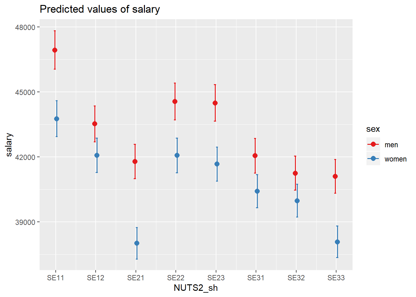
Figure 7: SSYK 214, Architects, engineers and related professionals, Year 2014 - 2018
plot(model, which = 1)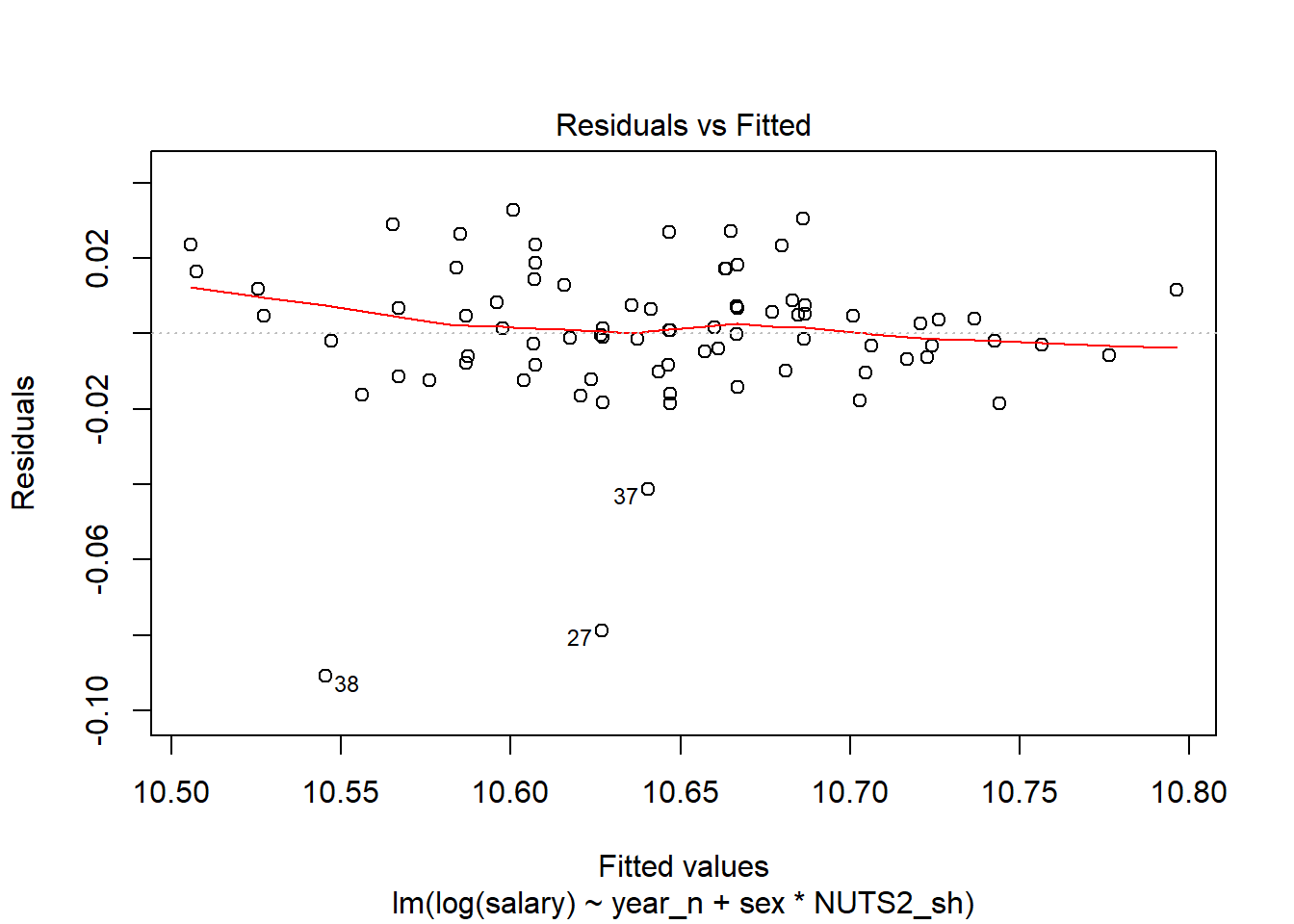
Figure 8: SSYK 214, Architects, engineers and related professionals, Year 2014 - 2018
tb[37,]## # A tibble: 1 x 11
## region sector `occuptional (~ sex year salary year_n NUTS2_sh fit
## <chr> <chr> <chr> <chr> <chr> <dbl> <dbl> <chr> <dbl>
## 1 SE21 ~ 0 all~ 214 Engineering~ men 2016 40100 2016 SE21 41037.
## # ... with 2 more variables: lwr <dbl>, upr <dbl>And the interaction between year and region. The F-value from the Anova table for the region is 0,57 (Pr(>F) < 0,77) implying no significant relation.
model <-lm (log(salary) ~ year_n * NUTS2_sh + sex , data = tb)

summary(model) %>%
  tidy() %>%
  knitr::kable(
  booktabs = TRUE,
caption = 'Summary from linear model fit')| term | estimate | std.error | statistic | p.value |
|---|---|---|---|---|
| (Intercept) | -32.1955668 | 10.7951966 | -2.9823975 | 0.0040635 |
| year_n | 0.0213028 | 0.0053548 | 3.9782933 | 0.0001818 |
| NUTS2_shSE12 | -4.0204905 | 15.2667129 | -0.2633501 | 0.7931402 |
| NUTS2_shSE21 | 0.6481345 | 15.2667129 | 0.0424541 | 0.9662710 |
| NUTS2_shSE22 | 18.2873103 | 15.2667129 | 1.1978551 | 0.2354607 |
| NUTS2_shSE23 | 7.7565167 | 15.2667129 | 0.5080672 | 0.6131806 |
| NUTS2_shSE31 | -5.4895464 | 15.2667129 | -0.3595762 | 0.7203666 |
| NUTS2_shSE32 | -3.2845607 | 15.2667129 | -0.2151452 | 0.8303490 |
| NUTS2_shSE33 | 9.2276482 | 15.2667129 | 0.6044293 | 0.5477290 |
| sexwomen | -0.0587056 | 0.0053548 | -10.9632632 | 0.0000000 |
| year_n:NUTS2_shSE12 | 0.0019658 | 0.0075728 | 0.2595848 | 0.7960305 |
| year_n:NUTS2_shSE21 | -0.0003853 | 0.0075728 | -0.0508802 | 0.9595820 |
| year_n:NUTS2_shSE22 | -0.0090938 | 0.0075728 | -1.2008536 | 0.2343036 |
| year_n:NUTS2_shSE23 | -0.0038730 | 0.0075728 | -0.5114312 | 0.6108371 |
| year_n:NUTS2_shSE31 | 0.0026760 | 0.0075728 | 0.3533662 | 0.7249937 |
| year_n:NUTS2_shSE32 | 0.0015747 | 0.0075728 | 0.2079419 | 0.8359451 |
| year_n:NUTS2_shSE33 | -0.0046447 | 0.0075728 | -0.6133392 | 0.5418602 |
summary(model)$r.squared## [1] 0.8888956Anova(model, type=2) %>%
tidy() %>%
knitr::kable(
booktabs = TRUE,
caption = 'Anova report from linear model fit')| term | sumsq | df | statistic | p.value |
|---|---|---|---|---|
| year_n | 0.0629183 | 1 | 109.7152945 | 0.0000000 |
| NUTS2_sh | 0.1548911 | 7 | 38.5850132 | 0.0000000 |
| sex | 0.0689270 | 1 | 120.1931409 | 0.0000000 |
| year_n:NUTS2_sh | 0.0023115 | 7 | 0.5758246 | 0.7728945 |
| Residuals | 0.0361285 | 63 | NA | NA |
plot_model(model, type = "pred", terms = c("NUTS2_sh", "year_n"))## Model has log-transformed response. Back-transforming predictions to original response scale. Standard errors are still on the log-scale.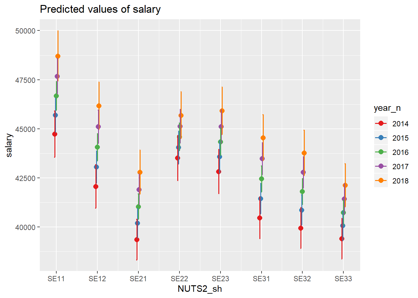
Figure 9: SSYK 214, Architects, engineers and related professionals, Year 2014 - 2018
plot(model, which = 1)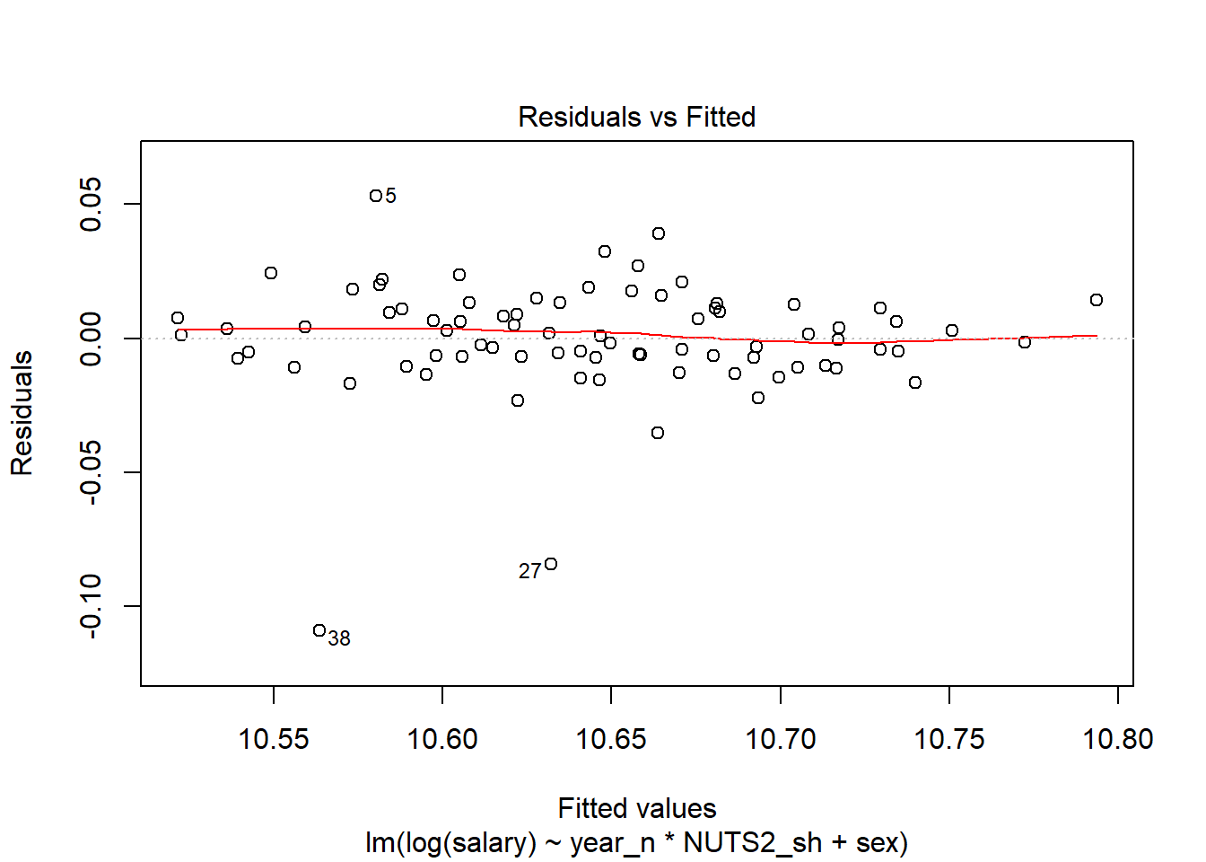
Figure 10: SSYK 214, Architects, engineers and related professionals, Year 2014 - 2018
Finally the interaction between gender, year and region, the only significant interaction is between the region and gender, F-value from the Anova table for the interaction is 2,4 (Pr(>F) < 0.033)
model <-lm (log(salary) ~ year_n * NUTS2_sh * sex , data = tb)

summary(model) %>%
  tidy() %>%
  knitr::kable(
  booktabs = TRUE,
caption = 'Summary from linear model fit')| term | estimate | std.error | statistic | p.value |
|---|---|---|---|---|
| (Intercept) | -34.6715204 | 14.5497427 | -2.3829645 | 0.0211805 |
| year_n | 0.0225338 | 0.0072171 | 3.1222585 | 0.0030380 |
| NUTS2_shSE12 | 5.2021839 | 20.5764435 | 0.2528223 | 0.8014851 |
| NUTS2_shSE21 | 5.5082002 | 20.5764435 | 0.2676945 | 0.7900815 |
| NUTS2_shSE22 | 25.5308721 | 20.5764435 | 1.2407816 | 0.2207168 |
| NUTS2_shSE23 | 16.1162328 | 20.5764435 | 0.7832370 | 0.4373355 |
| NUTS2_shSE31 | -18.4371634 | 20.5764435 | -0.8960326 | 0.3747072 |
| NUTS2_shSE32 | 7.6855067 | 20.5764435 | 0.3735100 | 0.7104136 |
| NUTS2_shSE33 | 5.0530040 | 20.5764435 | 0.2455723 | 0.8070603 |
| sexwomen | 4.8932017 | 20.5764435 | 0.2378060 | 0.8130438 |
| year_n:NUTS2_shSE12 | -0.0026179 | 0.0102066 | -0.2564919 | 0.7986672 |
| year_n:NUTS2_shSE21 | -0.0027899 | 0.0102066 | -0.2733393 | 0.7857651 |
| year_n:NUTS2_shSE22 | -0.0126899 | 0.0102066 | -1.2433117 | 0.2197916 |
| year_n:NUTS2_shSE23 | -0.0080207 | 0.0102066 | -0.7858392 | 0.4358239 |
| year_n:NUTS2_shSE31 | 0.0090909 | 0.0102066 | 0.8906917 | 0.3775375 |
| year_n:NUTS2_shSE32 | -0.0038764 | 0.0102066 | -0.3797940 | 0.7057736 |
| year_n:NUTS2_shSE33 | -0.0025723 | 0.0102066 | -0.2520253 | 0.8020975 |
| year_n:sexwomen | -0.0024619 | 0.0102066 | -0.2412080 | 0.8104213 |
| NUTS2_shSE12:sexwomen | -18.4453487 | 29.0994854 | -0.6338720 | 0.5291736 |
| NUTS2_shSE21:sexwomen | -9.7201315 | 29.0994854 | -0.3340310 | 0.7398112 |
| NUTS2_shSE22:sexwomen | -14.4871236 | 29.0994854 | -0.4978481 | 0.6208644 |
| NUTS2_shSE23:sexwomen | -16.7194322 | 29.0994854 | -0.5745611 | 0.5682714 |
| NUTS2_shSE31:sexwomen | 25.8952341 | 29.0994854 | 0.8898863 | 0.3779654 |
| NUTS2_shSE32:sexwomen | -21.9401348 | 29.0994854 | -0.7539699 | 0.4545502 |
| NUTS2_shSE33:sexwomen | 8.3492884 | 29.0994854 | 0.2869222 | 0.7754068 |
| year_n:NUTS2_shSE12:sexwomen | 0.0091674 | 0.0144343 | 0.6351107 | 0.5283723 |
| year_n:NUTS2_shSE21:sexwomen | 0.0048091 | 0.0144343 | 0.3331727 | 0.7404549 |
| year_n:NUTS2_shSE22:sexwomen | 0.0071923 | 0.0144343 | 0.4982800 | 0.6205623 |
| year_n:NUTS2_shSE23:sexwomen | 0.0082955 | 0.0144343 | 0.5747113 | 0.5681705 |
| year_n:NUTS2_shSE31:sexwomen | -0.0128299 | 0.0144343 | -0.8888492 | 0.3785170 |
| year_n:NUTS2_shSE32:sexwomen | 0.0109022 | 0.0144343 | 0.7552986 | 0.4537602 |
| year_n:NUTS2_shSE33:sexwomen | -0.0041447 | 0.0144343 | -0.2871452 | 0.7752371 |
summary(model)$r.squared## [1] 0.9231133Anova(model, type=2) %>%
tidy() %>%
knitr::kable(
booktabs = TRUE,
caption = 'Anova report from linear model fit')| term | sumsq | df | statistic | p.value |
|---|---|---|---|---|
| year_n | 0.0629183 | 1 | 120.7946290 | 0.0000000 |
| NUTS2_sh | 0.1637127 | 14 | 22.4504512 | 0.0000000 |
| sex | 0.0777463 | 8 | 18.6578050 | 0.0000000 |
| year_n:NUTS2_sh | 0.0023115 | 7 | 0.6339728 | 0.7254512 |
| year_n:sex | 0.0000085 | 1 | 0.0163969 | 0.8986442 |
| NUTS2_sh:sex | 0.0088184 | 7 | 2.4186030 | 0.0332038 |
| year_n:NUTS2_sh:sex | 0.0022998 | 7 | 0.6307550 | 0.7280524 |
| Residuals | 0.0250018 | 48 | NA | NA |
plot_model(model, type = "pred", terms = c("NUTS2_sh", "year_n", "sex"))## Model has log-transformed response. Back-transforming predictions to original response scale. Standard errors are still on the log-scale.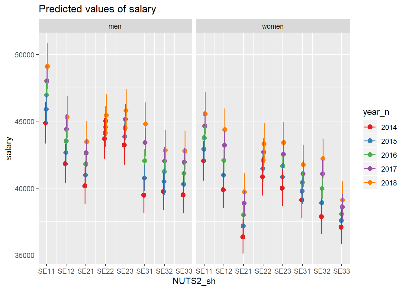
Figure 11: SSYK 214, Architects, engineers and related professionals, Year 2014 - 2018
plot(model, which = 1)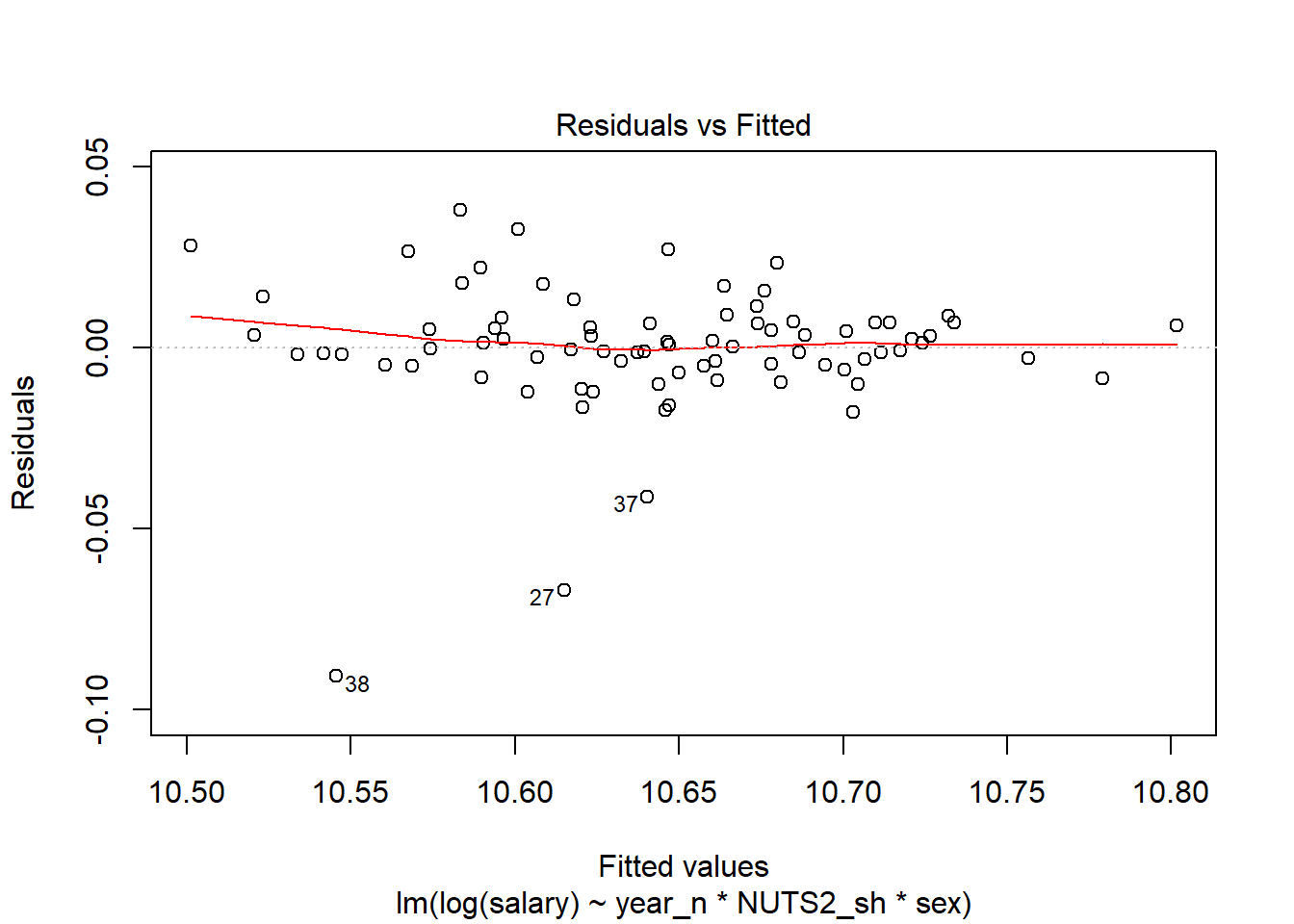
Figure 12: SSYK 214, Architects, engineers and related professionals, Year 2014 - 2018