In my last post, I found that the region has a significant impact on the salary of engineers. Is the significance of the region unique to engineers or are there similar correlations in other occupational groups?
Statistics Sweden use NUTS (Nomenclature des Unités Territoriales Statistiques), which is the EU’s hierarchical regional division, to specify the regions.
The F-value from the Anova table is used as the single value to discriminate how much the region and salary correlates. For exploratory analysis, the Anova value seems good enough.
First, define libraries and functions.
library (tidyverse) ## -- Attaching packages -------------------------------------- tidyverse 1.3.0 --## v ggplot2 3.2.1 v purrr 0.3.3
## v tibble 2.1.3 v dplyr 0.8.3
## v tidyr 1.0.2 v stringr 1.4.0
## v readr 1.3.1 v forcats 0.4.0## -- Conflicts ----------------------------------------- tidyverse_conflicts() --
## x dplyr::filter() masks stats::filter()
## x dplyr::lag() masks stats::lag()library (broom)
library (car)## Loading required package: carData##
## Attaching package: 'car'## The following object is masked from 'package:dplyr':
##
## recode## The following object is masked from 'package:purrr':
##
## somelibrary (swemaps) # devtools::install_github('reinholdsson/swemaps')
library(sjPlot)## Registered S3 methods overwritten by 'lme4':
## method from
## cooks.distance.influence.merMod car
## influence.merMod car
## dfbeta.influence.merMod car
## dfbetas.influence.merMod car## Install package "strengejacke" from GitHub (`devtools::install_github("strengejacke/strengejacke")`) to load all sj-packages at once!readfile <- function (file1){
read_csv (file1, col_types = cols(), locale = readr::locale (encoding = "latin1"), na = c("..", "NA")) %>%
gather (starts_with("19"), starts_with("20"), key = "year", value = salary) %>%
drop_na() %>%
mutate (year_n = parse_number (year))
}
nuts <- read.csv("nuts.csv") %>%
mutate(NUTS2_sh = substr(NUTS2, 1, 4))
nuts %>%
distinct (NUTS2_en) %>%
knitr::kable(
booktabs = TRUE,
caption = 'Nomenclature des Unités Territoriales Statistiques (NUTS)')| NUTS2_en |
|---|
| SE11 Stockholm |
| SE12 East-Central Sweden |
| SE21 Småland and islands |
| SE22 South Sweden |
| SE23 West Sweden |
| SE31 North-Central Sweden |
| SE32 Central Norrland |
| SE33 Upper Norrland |
map_ln_n <- map_ln %>%
  mutate(lnkod_n = as.numeric(lnkod))
The data table is downloaded from Statistics Sweden. It is saved as a comma-delimited file without heading, 000000CG.csv, http://www.statistikdatabasen.scb.se/pxweb/en/ssd/.
The table: Average basic salary, monthly salary and women´s salary as a percentage of men´s salary by region, sector, occupational group (SSYK 2012) and sex. Year 2014 - 2018 Monthly salary All sectors
In the plot and tables, you can also find information on how the increase in salaries per year for each occupational group is affected when the interactions are taken into account.
tb <- readfile ("000000CG.csv") %>%
  left_join(nuts %>% distinct (NUTS2_en, NUTS2_sh), by = c("region" = "NUTS2_en"))
## Warning: Column `region`/`NUTS2_en` joining character vector and factor,
## coercing into character vectortb_map <- readfile ("000000CG.csv") %>%
left_join(nuts, by = c("region" = "NUTS2_en")) %>%
right_join(map_ln_n, by = c("Länskod" = "lnkod_n"))## Warning: Column `region`/`NUTS2_en` joining character vector and factor,
## coercing into character vectorsummary_table = vector()
anova_table = vector()
for (i in unique(tb$`occuptional (SSYK 2012)`)){
temp <- filter(tb, `occuptional (SSYK 2012)` == i)
if (dim(temp)[1] > 75){
model <- lm(log(salary) ~ region + sex + year_n, data = temp)
summary_table <- rbind (summary_table, mutate (tidy (summary (model)), ssyk = i, interaction = "none"))
anova_table <- rbind (anova_table, mutate (tidy (Anova (model, type = 2)), ssyk = i, interaction = "none"))
model <- lm(log(salary) ~ region * sex + year_n, data = temp)
summary_table <- rbind (summary_table, mutate (tidy (summary (model)), ssyk = i, interaction = "region and sex"))
anova_table <- rbind (anova_table, mutate (tidy (Anova (model, type = 2)), ssyk = i, interaction = "region and sex"))
model <- lm(log(salary) ~ region * year_n + sex, data = temp)
summary_table <- rbind (summary_table, mutate (tidy (summary (model)), ssyk = i, interaction = "region and year"))
anova_table <- rbind (anova_table, mutate (tidy (Anova (model, type = 2)), ssyk = i, interaction = "region and year"))
model <- lm(log(salary) ~ region * year_n * sex, data = temp)
summary_table <- rbind (summary_table, mutate (tidy (summary (model)), ssyk = i, interaction = "region, year and sex"))
anova_table <- rbind (anova_table, mutate (tidy (Anova (model, type = 2)), ssyk = i, interaction = "region, year and sex"))
}
}## Note: model has aliased coefficients
## sums of squares computed by model comparison
## Note: model has aliased coefficients
## sums of squares computed by model comparisonanova_table <- anova_table %>% rowwise() %>% mutate(contcol = str_count(term, ":"))
summary_table <- summary_table %>% rowwise() %>% mutate(contcol = str_count(term, ":"))
merge(summary_table, anova_table, by = c("ssyk", "interaction"), all = TRUE) %>%
filter (term.x == "year_n") %>%
filter (term.y == "region") %>%
filter (interaction == "none") %>%
mutate (estimate = (exp(estimate) - 1) * 100) %>%
ggplot () +
geom_point (mapping = aes(x = estimate, y = statistic.y, colour = interaction)) +
labs(
x = "Increase in salaries (% / year)",
y = "F-value for interaction"
) 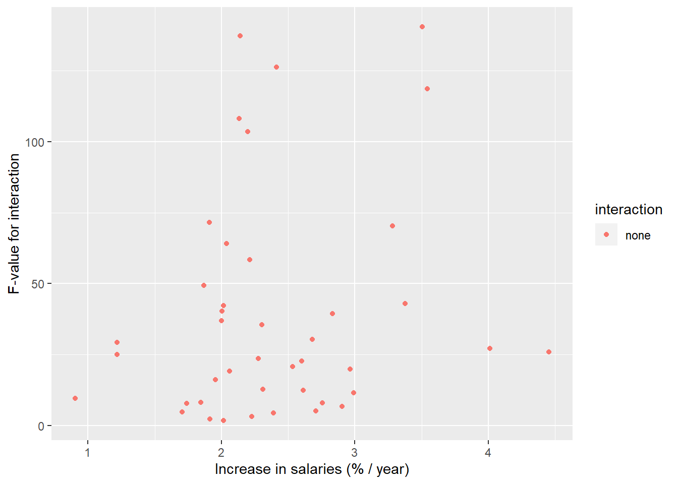
Figure 1: The significance of the region on the salary in Sweden, a comparison between different occupational groups, Year 2014 - 2018
merge(summary_table, anova_table, by = c("ssyk", "interaction"), all = TRUE) %>%
  filter (term.x == "year_n") %>%
  filter (contcol.y > 0) %>%
  # only look at the interactions between all three variables in the case with interaction region, year and sex
  filter (!(contcol.y == 1 & interaction == "region, year and sex")) %>%

  mutate (estimate = (exp(estimate) - 1) * 100) %>%
  ggplot () +
    geom_point (mapping = aes(x = estimate, y = statistic.y, colour = interaction)) +
    labs(
      x = "Increase in salaries (% / year)",
      y = "F-value for interaction"
) 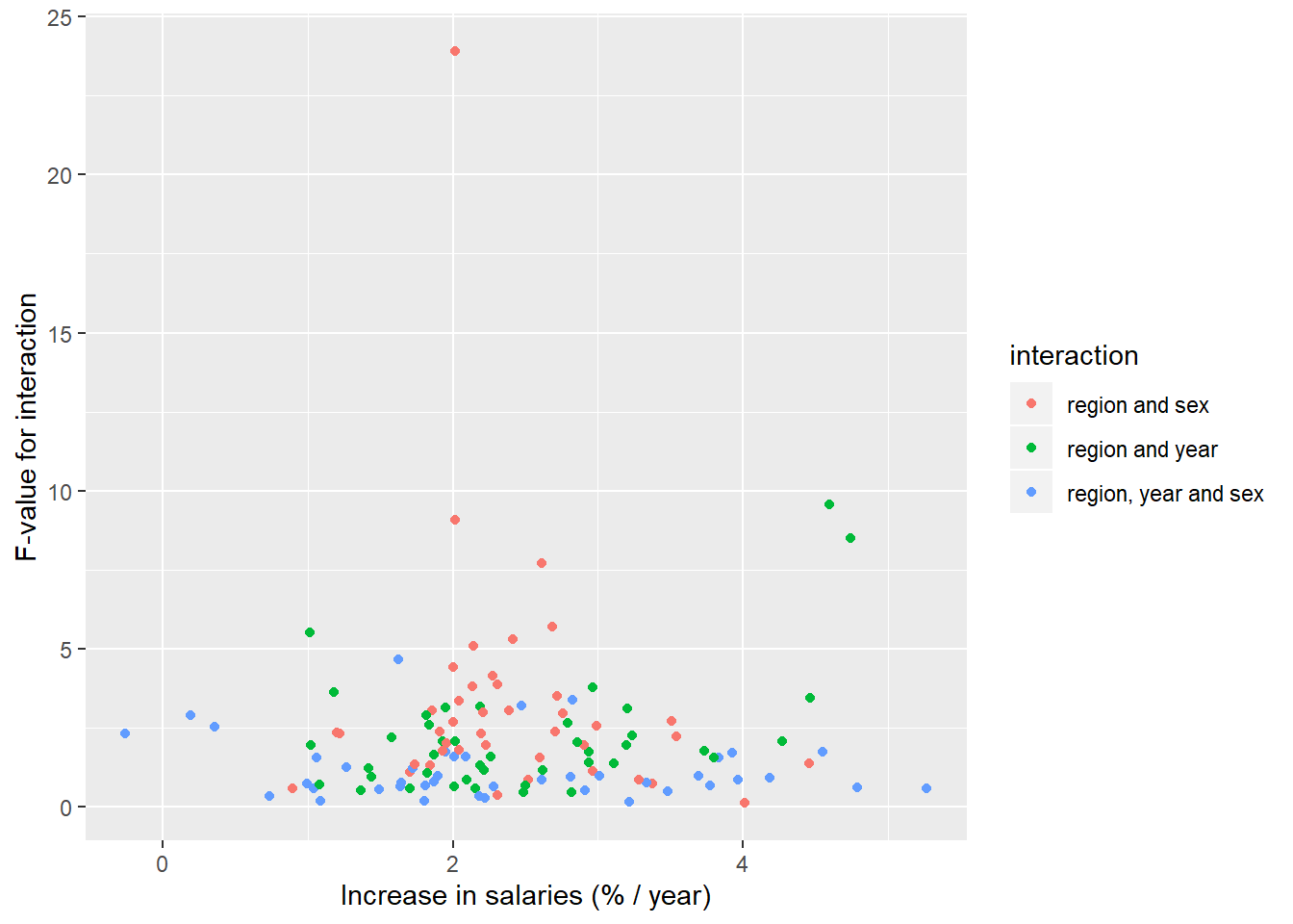
Figure 2: The significance of the interaction between region, year and sex on the salary in Sweden, a comparison between different occupational groups, Year 2014 - 2018
The tables with all occupational groups sorted by F-value in descending order.
merge(summary_table, anova_table, c("ssyk", "interaction"), all = TRUE) %>%
  filter (term.x == "year_n") %>%
  filter (term.y == "region") %>%
  filter (interaction == "none") %>%
  mutate (estimate = (exp(estimate) - 1) * 100) %>%
  select (ssyk, estimate, statistic.y, interaction) %>%
  rename (`F-value for age` = statistic.y) %>%
  rename (`Increase in salary` = estimate) %>%
  arrange (desc (`F-value for age`)) %>%
  knitr::kable(
    booktabs = TRUE,
caption = 'Correlation for F-value (region) and the yearly increase in salaries')| ssyk | Increase in salary | F-value for age | interaction |
|---|---|---|---|
| 234 Primary- and pre-school teachers | 3.505364 | 140.459561 | none |
| 242 Organisation analysts, policy administrators and human resource specialists | 2.141124 | 137.227070 | none |
| 159 Other social services managers | 2.412305 | 126.200697 | none |
| 141 Primary and secondary schools and adult education managers | 3.543591 | 118.692580 | none |
| 335 Tax and related government associate professionals | 2.133970 | 108.141526 | none |
| 251 ICT architects, systems analysts and test managers | 2.196568 | 103.500079 | none |
| 332 Insurance advisers, sales and purchasing agents | 1.910500 | 71.550568 | none |
| 336 Police officers | 3.280076 | 70.269911 | none |
| 241 Accountants, financial analysts and fund managers | 2.040018 | 64.180404 | none |
| 235 Teaching professionals not elsewhere classified | 2.210947 | 58.449386 | none |
| 351 ICT operations and user support technicians | 1.868739 | 49.435480 | none |
| 233 Secondary education teachers | 3.377886 | 43.017847 | none |
| 331 Financial and accounting associate professionals | 2.016965 | 42.321607 | none |
| 214 Engineering professionals | 2.002819 | 40.294194 | none |
| 218 Specialists within environmental and health protection | 2.831305 | 39.372062 | none |
| 533 Health care assistants | 2.001888 | 36.961185 | none |
| 261 Legal professionals | 2.304699 | 35.545371 | none |
| 231 University and higher education teachers | 2.682606 | 30.352218 | none |
| 243 Marketing and public relations professionals | 1.217703 | 29.319658 | none |
| 222 Nursing professionals | 4.012209 | 27.254061 | none |
| 123 Administration and planning managers | 4.455192 | 25.902695 | none |
| 264 Authors, journalists and linguists | 1.218409 | 24.973290 | none |
| 531 Child care workers and teachers aides | 2.276723 | 23.659505 | none |
| 333 Business services agents | 2.601340 | 22.810204 | none |
| 311 Physical and engineering science technicians | 2.532877 | 20.769863 | none |
| 266 Social work and counselling professionals | 2.965491 | 19.825931 | none |
| 411 Office assistants and other secretaries | 2.060828 | 19.127036 | none |
| 534 Attendants, personal assistants and related workers | 1.956992 | 16.198710 | none |
| 341 Social work and religious associate professionals | 2.309857 | 12.736283 | none |
| 321 Medical and pharmaceutical technicians | 2.613786 | 12.424504 | none |
| 232 Vocational education teachers | 2.990624 | 11.524474 | none |
| 221 Medical doctors | 0.902755 | 9.634942 | none |
| 422 Client information clerks | 1.843752 | 8.137514 | none |
| 512 Cooks and cold-buffet managers | 2.756431 | 8.061511 | none |
| 962 Newspaper distributors, janitors and other service workers | 1.740067 | 7.765145 | none |
| 522 Shop staff | 2.903890 | 6.830648 | none |
| 532 Personal care workers in health services | 2.705999 | 5.078780 | none |
| 432 Stores and transport clerks | 1.705670 | 4.865026 | none |
| 541 Other surveillance and security workers | 2.389682 | 4.371317 | none |
| 941 Fast-food workers, food preparation assistants | 2.227375 | 3.219358 | none |
| 833 Heavy truck and bus drivers | 1.912077 | 2.247326 | none |
| 911 Cleaners and helpers | 2.016100 | 1.711840 | none |
merge(summary_table, anova_table, c("ssyk", "interaction"), all = TRUE) %>%
  filter (term.x == "year_n") %>%
  filter (contcol.y > 0) %>%
  filter (interaction == "region and sex") %>%
  mutate (estimate = (exp(estimate) - 1) * 100) %>%
  select (ssyk, estimate, statistic.y, interaction) %>%
  rename (`F-value for age` = statistic.y) %>%
  rename (`Increase in salary` = estimate) %>%
  arrange (desc (`F-value for age`)) %>%
  knitr::kable(
    booktabs = TRUE,
caption = 'Correlation for F-value (region and sex) and the yearly increase in salaries')| ssyk | Increase in salary | F-value for age | interaction |
|---|---|---|---|
| 331 Financial and accounting associate professionals | 2.0169648 | 23.9056822 | region and sex |
| 911 Cleaners and helpers | 2.0160997 | 9.0815382 | region and sex |
| 321 Medical and pharmaceutical technicians | 2.6137864 | 7.7168336 | region and sex |
| 231 University and higher education teachers | 2.6826060 | 5.6873851 | region and sex |
| 159 Other social services managers | 2.4123053 | 5.3090755 | region and sex |
| 242 Organisation analysts, policy administrators and human resource specialists | 2.1411239 | 5.0798948 | region and sex |
| 533 Health care assistants | 2.0018877 | 4.4194926 | region and sex |
| 531 Child care workers and teachers aides | 2.2767234 | 4.1363582 | region and sex |
| 261 Legal professionals | 2.3101043 | 3.8795657 | region and sex |
| 335 Tax and related government associate professionals | 2.1339700 | 3.8162101 | region and sex |
| 218 Specialists within environmental and health protection | 2.7191768 | 3.4940939 | region and sex |
| 241 Accountants, financial analysts and fund managers | 2.0400185 | 3.3402726 | region and sex |
| 541 Other surveillance and security workers | 2.3896824 | 3.0479843 | region and sex |
| 351 ICT operations and user support technicians | 1.8593806 | 3.0366516 | region and sex |
| 235 Teaching professionals not elsewhere classified | 2.2109466 | 2.9986405 | region and sex |
| 512 Cooks and cold-buffet managers | 2.7564313 | 2.9661198 | region and sex |
| 234 Primary- and pre-school teachers | 3.5053638 | 2.7061253 | region and sex |
| 214 Engineering professionals | 2.0028190 | 2.6793275 | region and sex |
| 232 Vocational education teachers | 2.9906243 | 2.5473580 | region and sex |
| 532 Personal care workers in health services | 2.7059985 | 2.3861956 | region and sex |
| 332 Insurance advisers, sales and purchasing agents | 1.9105004 | 2.3851151 | region and sex |
| 243 Marketing and public relations professionals | 1.2005440 | 2.3538771 | region and sex |
| 264 Authors, journalists and linguists | 1.2184087 | 2.3283437 | region and sex |
| 251 ICT architects, systems analysts and test managers | 2.1965679 | 2.3071242 | region and sex |
| 141 Primary and secondary schools and adult education managers | 3.5435906 | 2.2283878 | region and sex |
| 534 Attendants, personal assistants and related workers | 1.9569919 | 2.0176966 | region and sex |
| 941 Fast-food workers, food preparation assistants | 2.2273749 | 1.9439585 | region and sex |
| 522 Shop staff | 2.9038903 | 1.9435000 | region and sex |
| 411 Office assistants and other secretaries | 2.0399065 | 1.8087907 | region and sex |
| 833 Heavy truck and bus drivers | 1.9298918 | 1.7646741 | region and sex |
| 333 Business services agents | 2.6013400 | 1.5532994 | region and sex |
| 123 Administration and planning managers | 4.4564515 | 1.3795888 | region and sex |
| 962 Newspaper distributors, janitors and other service workers | 1.7400674 | 1.3302289 | region and sex |
| 422 Client information clerks | 1.8437523 | 1.3111491 | region and sex |
| 266 Social work and counselling professionals | 2.9654913 | 1.1228380 | region and sex |
| 432 Stores and transport clerks | 1.7056704 | 1.0829037 | region and sex |
| 311 Physical and engineering science technicians | 2.5162972 | 0.8523619 | region and sex |
| 336 Police officers | 3.2800755 | 0.8458087 | region and sex |
| 233 Secondary education teachers | 3.3778859 | 0.7369872 | region and sex |
| 221 Medical doctors | 0.8945233 | 0.5918577 | region and sex |
| 341 Social work and religious associate professionals | 2.3098566 | 0.3654042 | region and sex |
| 222 Nursing professionals | 4.0122087 | 0.1103390 | region and sex |
merge(summary_table, anova_table, c("ssyk", "interaction"), all = TRUE) %>%
  filter (term.x == "year_n") %>%
  filter (contcol.y > 0) %>%
  filter (interaction == "region and year") %>%
  mutate (estimate = (exp(estimate) - 1) * 100) %>%
  select (ssyk, estimate, statistic.y, interaction) %>%
  rename (`F-value for age` = statistic.y) %>%
  rename (`Increase in salary` = estimate) %>%
  arrange (desc (`F-value for age`)) %>%
  knitr::kable(
    booktabs = TRUE,
caption = 'Correlation for F-value (region and year) and the yearly increase in salaries')| ssyk | Increase in salary | F-value for age | interaction |
|---|---|---|---|
| 222 Nursing professionals | 4.594527 | 9.5756908 | region and year |
| 234 Primary- and pre-school teachers | 4.741438 | 8.4929762 | region and year |
| 962 Newspaper distributors, janitors and other service workers | 1.014436 | 5.5221538 | region and year |
| 218 Specialists within environmental and health protection | 2.960551 | 3.7726084 | region and year |
| 341 Social work and religious associate professionals | 1.179665 | 3.6377998 | region and year |
| 141 Primary and secondary schools and adult education managers | 4.464391 | 3.4565788 | region and year |
| 231 University and higher education teachers | 2.190339 | 3.1807419 | region and year |
| 531 Child care workers and teachers aides | 1.946134 | 3.1384371 | region and year |
| 123 Administration and planning managers | 3.202935 | 3.0929465 | region and year |
| 351 ICT operations and user support technicians | 1.818022 | 2.8907900 | region and year |
| 335 Tax and related government associate professionals | 2.794241 | 2.6351058 | region and year |
| 311 Physical and engineering science technicians | 1.836449 | 2.5772805 | region and year |
| 336 Police officers | 3.238027 | 2.2608889 | region and year |
| 221 Medical doctors | 1.577680 | 2.1873354 | region and year |
| 266 Social work and counselling professionals | 4.269070 | 2.0856790 | region and year |
| 534 Attendants, personal assistants and related workers | 2.012733 | 2.0738388 | region and year |
| 333 Business services agents | 1.929570 | 2.0713461 | region and year |
| 532 Personal care workers in health services | 2.854891 | 2.0354065 | region and year |
| 264 Authors, journalists and linguists | 1.020091 | 1.9403580 | region and year |
| 332 Insurance advisers, sales and purchasing agents | 3.197316 | 1.9390313 | region and year |
| 232 Vocational education teachers | 3.729880 | 1.7811629 | region and year |
| 512 Cooks and cold-buffet managers | 2.937534 | 1.7459584 | region and year |
| 411 Office assistants and other secretaries | 1.870052 | 1.6496037 | region and year |
| 235 Teaching professionals not elsewhere classified | 2.263332 | 1.5866915 | region and year |
| 233 Secondary education teachers | 3.800949 | 1.5667053 | region and year |
| 159 Other social services managers | 2.939365 | 1.3862925 | region and year |
| 241 Accountants, financial analysts and fund managers | 3.112492 | 1.3754541 | region and year |
| 251 ICT architects, systems analysts and test managers | 2.189907 | 1.2977035 | region and year |
| 941 Fast-food workers, food preparation assistants | 1.418897 | 1.2189448 | region and year |
| 261 Legal professionals | 2.620417 | 1.1684118 | region and year |
| 242 Organisation analysts, policy administrators and human resource specialists | 2.212719 | 1.1514498 | region and year |
| 833 Heavy truck and bus drivers | 1.823095 | 1.0719499 | region and year |
| 911 Cleaners and helpers | 1.438852 | 0.9563272 | region and year |
| 432 Stores and transport clerks | 2.093243 | 0.8517395 | region and year |
| 331 Financial and accounting associate professionals | 1.079578 | 0.7062153 | region and year |
| 522 Shop staff | 2.500507 | 0.6743597 | region and year |
| 533 Health care assistants | 2.008445 | 0.6349934 | region and year |
| 214 Engineering professionals | 2.153132 | 0.5758246 | region and year |
| 243 Marketing and public relations professionals | 1.702978 | 0.5743298 | region and year |
| 422 Client information clerks | 1.363946 | 0.5084936 | region and year |
| 321 Medical and pharmaceutical technicians | 2.820296 | 0.4615622 | region and year |
| 541 Other surveillance and security workers | 2.488850 | 0.4542178 | region and year |
merge(summary_table, anova_table, c("ssyk", "interaction"), all = TRUE) %>%
  filter (term.x == "year_n") %>%
  filter (contcol.y > 1) %>%
  filter (interaction == "region, year and sex") %>%
  filter (!(contcol.y == 1 & interaction == "region, year and sex")) %>%
  mutate (estimate = (exp(estimate) - 1) * 100) %>%
  select (ssyk, estimate, statistic.y, interaction) %>%
  rename (`F-value for age` = statistic.y) %>%
  rename (`Increase in salary` = estimate) %>%
  arrange (desc (`F-value for age`)) %>%
  knitr::kable(
    booktabs = TRUE,
caption = 'Correlation for F-value (region, year and sex) and the yearly increase in salaries')| ssyk | Increase in salary | F-value for age | interaction |
|---|---|---|---|
| 531 Child care workers and teachers aides | 1.6212785 | 4.6701912 | region, year and sex |
| 541 Other surveillance and security workers | 2.8239443 | 3.3698474 | region, year and sex |
| 218 Specialists within environmental and health protection | 2.4738659 | 3.2049100 | region, year and sex |
| 331 Financial and accounting associate professionals | 0.1908239 | 2.8847688 | region, year and sex |
| 351 ICT operations and user support technicians | 0.3582487 | 2.5229634 | region, year and sex |
| 221 Medical doctors | -0.2578495 | 2.3158388 | region, year and sex |
| 411 Office assistants and other secretaries | 1.9518139 | 1.7466381 | region, year and sex |
| 141 Primary and secondary schools and adult education managers | 4.5500329 | 1.7360681 | region, year and sex |
| 512 Cooks and cold-buffet managers | 3.9252389 | 1.7021536 | region, year and sex |
| 251 ICT architects, systems analysts and test managers | 2.0097672 | 1.5905499 | region, year and sex |
| 242 Organisation analysts, policy administrators and human resource specialists | 2.0886458 | 1.5752902 | region, year and sex |
| 941 Fast-food workers, food preparation assistants | 1.0629882 | 1.5615772 | region, year and sex |
| 232 Vocational education teachers | 3.8326506 | 1.5493239 | region, year and sex |
| 235 Teaching professionals not elsewhere classified | 1.2656111 | 1.2406770 | region, year and sex |
| 911 Cleaners and helpers | 1.7251553 | 1.2122343 | region, year and sex |
| 332 Insurance advisers, sales and purchasing agents | 3.6964107 | 0.9875563 | region, year and sex |
| 833 Heavy truck and bus drivers | 1.8960959 | 0.9786211 | region, year and sex |
| 532 Personal care workers in health services | 3.0120859 | 0.9603131 | region, year and sex |
| 335 Tax and related government associate professionals | 2.8095715 | 0.9471462 | region, year and sex |
| 266 Social work and counselling professionals | 4.1855410 | 0.9152029 | region, year and sex |
| 123 Administration and planning managers | 3.9661945 | 0.8530921 | region, year and sex |
| 159 Other social services managers | 2.6152072 | 0.8505913 | region, year and sex |
| 533 Health care assistants | 1.8690208 | 0.7855258 | region, year and sex |
| 231 University and higher education teachers | 1.6422359 | 0.7732961 | region, year and sex |
| 241 Accountants, financial analysts and fund managers | 3.3332928 | 0.7520525 | region, year and sex |
| 333 Business services agents | 0.9959201 | 0.7345545 | region, year and sex |
| 233 Secondary education teachers | 3.7756980 | 0.6833044 | region, year and sex |
| 534 Attendants, personal assistants and related workers | 1.8119543 | 0.6586806 | region, year and sex |
| 243 Marketing and public relations professionals | 1.6359856 | 0.6487796 | region, year and sex |
| 214 Engineering professionals | 2.2789556 | 0.6307550 | region, year and sex |
| 234 Primary- and pre-school teachers | 4.7865061 | 0.6132542 | region, year and sex |
| 264 Authors, journalists and linguists | 1.0415688 | 0.5809769 | region, year and sex |
| 222 Nursing professionals | 5.2654653 | 0.5702894 | region, year and sex |
| 962 Newspaper distributors, janitors and other service workers | 1.4942008 | 0.5531934 | region, year and sex |
| 522 Shop staff | 2.9107242 | 0.5165112 | region, year and sex |
| 321 Medical and pharmaceutical technicians | 3.4804846 | 0.4863120 | region, year and sex |
| 341 Social work and religious associate professionals | 0.7370630 | 0.3372004 | region, year and sex |
| 311 Physical and engineering science technicians | 2.1802298 | 0.3313909 | region, year and sex |
| 261 Legal professionals | 2.2233855 | 0.2620376 | region, year and sex |
| 432 Stores and transport clerks | 1.7998663 | 0.1870227 | region, year and sex |
| 422 Client information clerks | 1.0842242 | 0.1733253 | region, year and sex |
| 336 Police officers | 3.2164461 | 0.1482551 | region, year and sex |
Let’s check what we have found.
temp <- tb %>%
  filter(`occuptional  (SSYK 2012)` == "234 Primary- and pre-school teachers")

model <-lm (log(salary) ~ year_n + sex + NUTS2_sh, data = temp)

plot_model(model, type = "pred", terms = c("NUTS2_sh"))
## Model has log-transformed response. Back-transforming predictions to original response scale. Standard errors are still on the log-scale.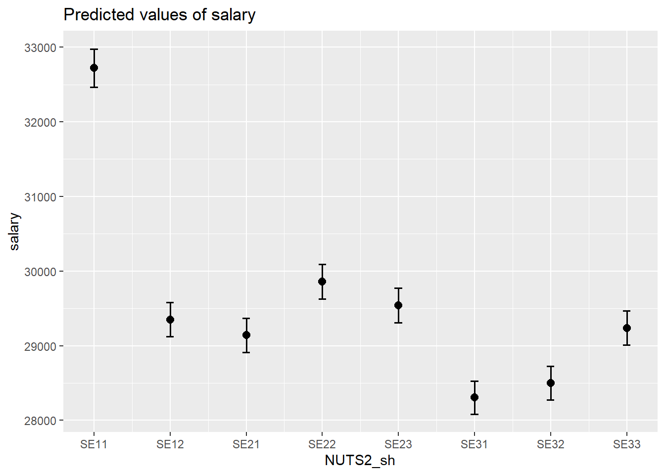
Figure 3: Highest F-value region, Primary- and pre-school teachers
tb_map %>%
    filter(`occuptional  (SSYK 2012)` == "234 Primary- and pre-school teachers") %>%
  ggplot() +
    geom_polygon(mapping = aes(x = ggplot_long, y = ggplot_lat, group = lnkod, fill = salary)) +
      facet_grid(. ~ year) +
coord_equal() 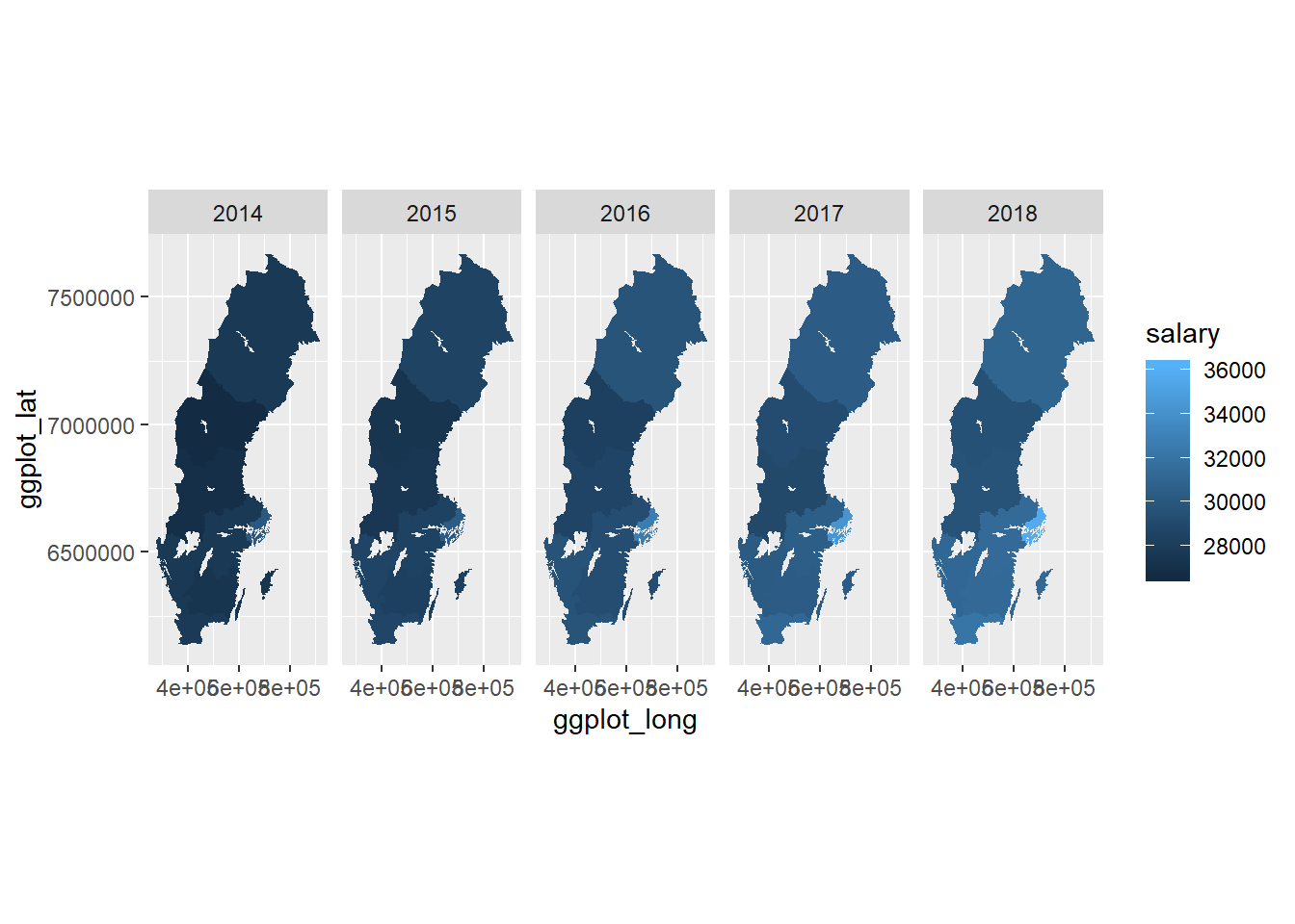
Figure 4: Highest F-value region, Primary- and pre-school teachers
temp <- tb %>%
  filter(`occuptional  (SSYK 2012)` == "911 Cleaners and helpers")

model <-lm (log(salary) ~ year_n + sex + NUTS2_sh, data = temp)

plot_model(model, type = "pred", terms = c("NUTS2_sh"))
## Model has log-transformed response. Back-transforming predictions to original response scale. Standard errors are still on the log-scale.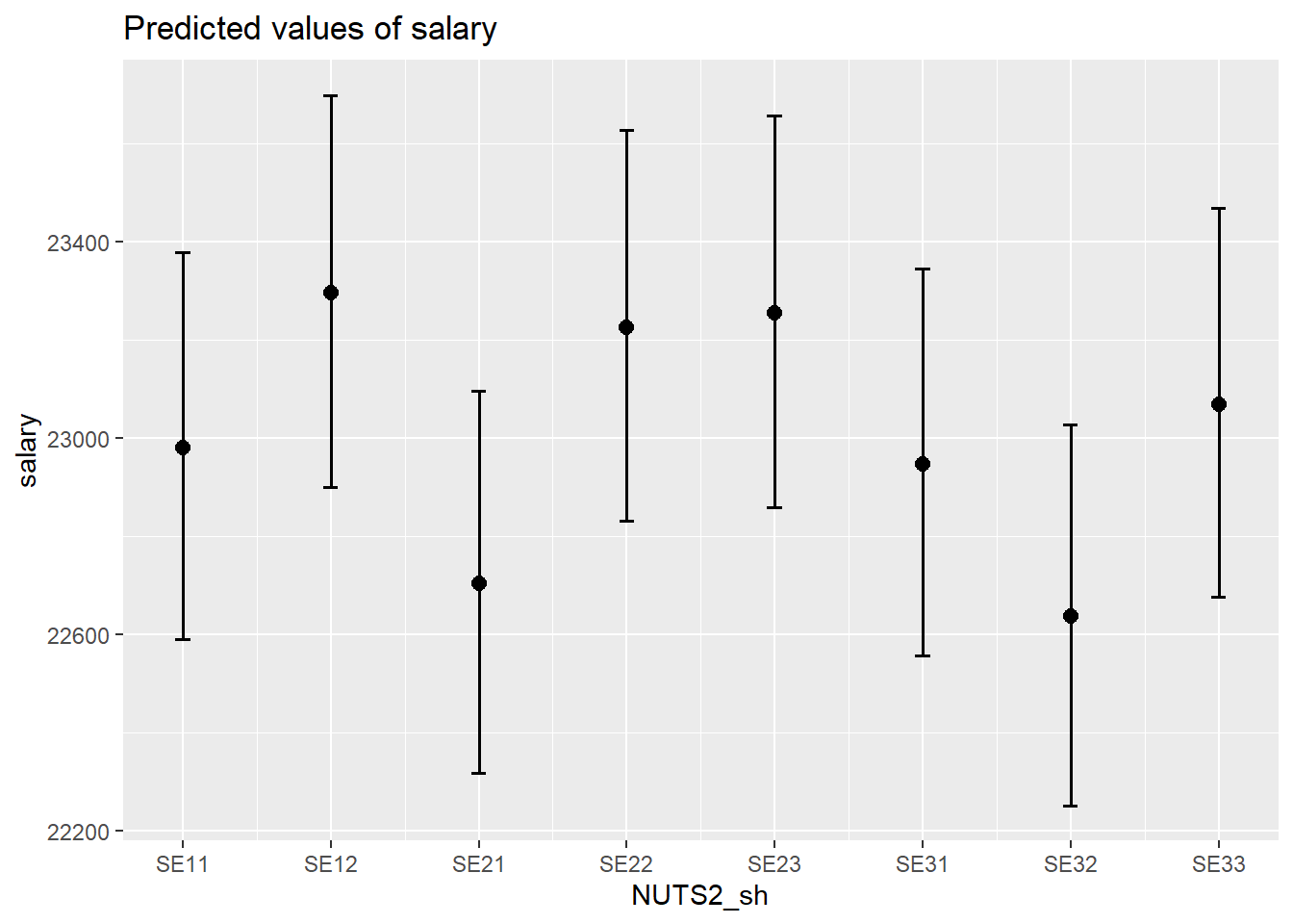
Figure 5: Lowest F-value region, Cleaners and helpers
temp <- tb %>%
  filter(`occuptional  (SSYK 2012)` == "331 Financial and accounting associate professionals")

model <-lm (log(salary) ~ year_n + sex * NUTS2_sh, data = temp)

plot_model(model, type = "pred", terms = c("NUTS2_sh", "sex"))
## Model has log-transformed response. Back-transforming predictions to original response scale. Standard errors are still on the log-scale.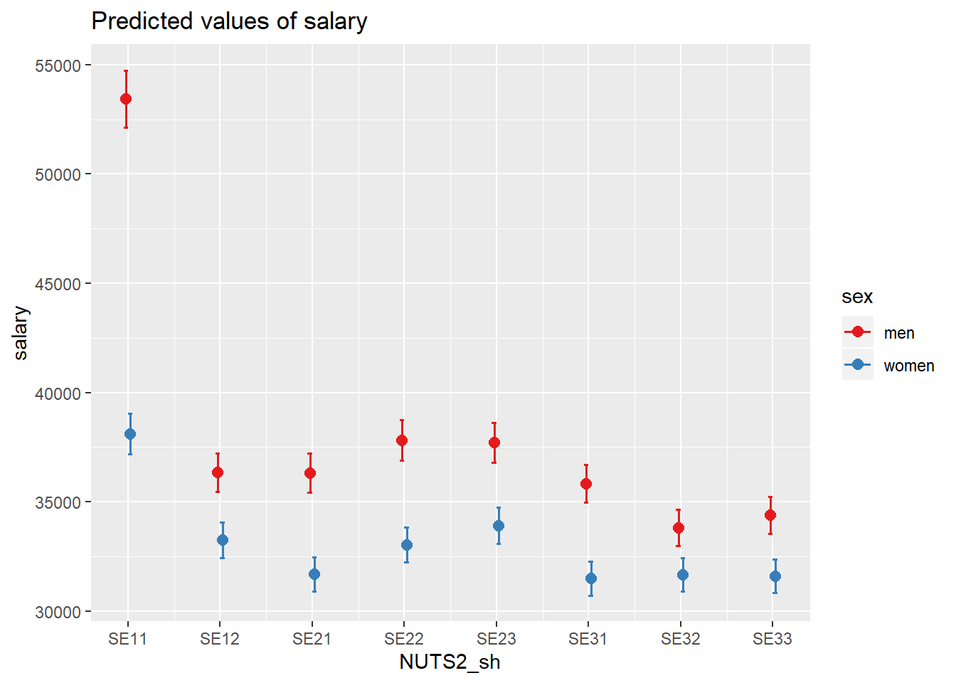
Figure 6: Highest F-value interaction gender and region, Financial and accounting associate professionals
tb_map %>%
    filter(`occuptional  (SSYK 2012)` == "331 Financial and accounting associate professionals") %>%
  filter (sex == "men") %>%
  ggplot() +
    geom_polygon(mapping = aes(x = ggplot_long, y = ggplot_lat, group = lnkod, fill = salary)) +
      facet_grid(. ~ year) +
coord_equal() 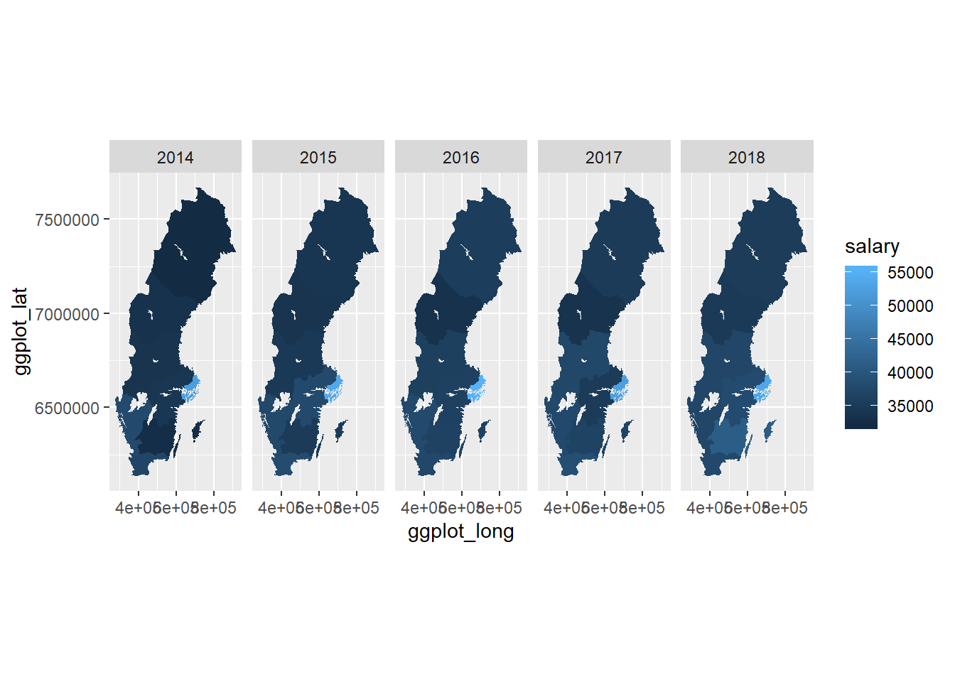
Figure 7: Highest F-value interaction gender and region, Financial and accounting associate professionals
tb_map %>%
    filter(`occuptional  (SSYK 2012)` == "331 Financial and accounting associate professionals") %>%
  filter (sex == "women") %>%
  ggplot() +
    geom_polygon(mapping = aes(x = ggplot_long, y = ggplot_lat, group = lnkod, fill = salary)) +
      facet_grid(. ~ year) +
coord_equal() 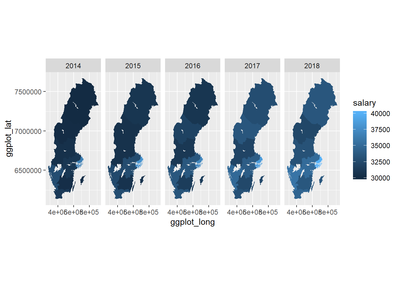
Figure 8: Highest F-value interaction gender and region, Financial and accounting associate professionals
temp <- tb %>%
  filter(`occuptional  (SSYK 2012)` == "222 Nursing professionals")

model <-lm (log(salary) ~ year_n + sex * NUTS2_sh, data = temp)

plot_model(model, type = "pred", terms = c("NUTS2_sh", "sex"))
## Model has log-transformed response. Back-transforming predictions to original response scale. Standard errors are still on the log-scale.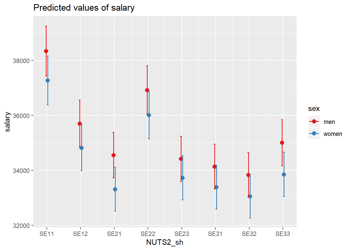
Figure 9: Lowest F-value interaction gender and region, Nursing professionals
temp <- tb %>%
  filter(`occuptional  (SSYK 2012)` == "222 Nursing professionals")

model <-lm (log(salary) ~ year_n * NUTS2_sh + sex , data = temp)

plot_model(model, type = "pred", terms = c("NUTS2_sh", "year_n"))
## Model has log-transformed response. Back-transforming predictions to original response scale. Standard errors are still on the log-scale.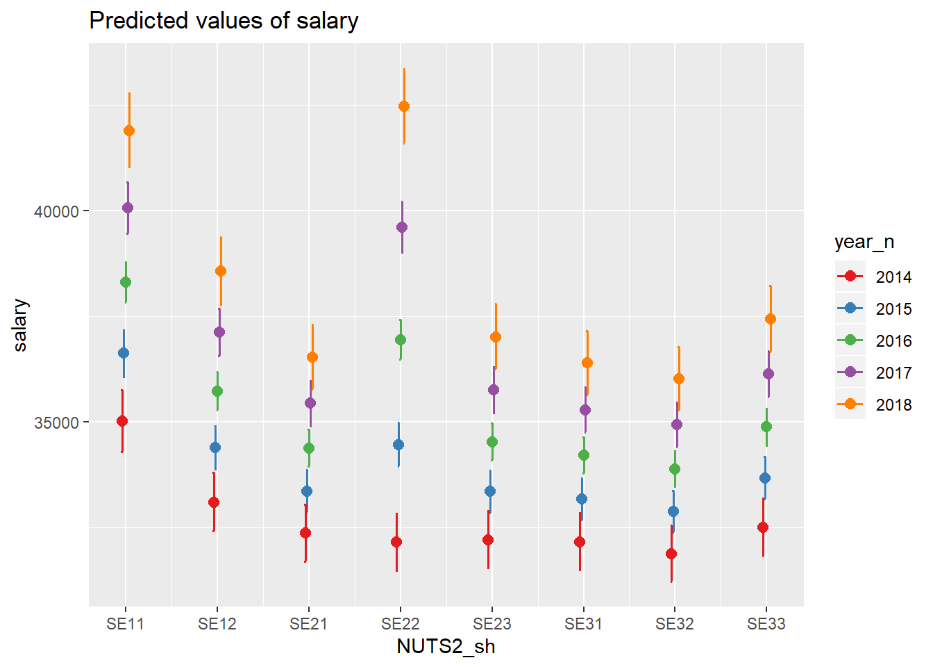
Figure 10: Highest F-value interaction year and region, Nursing professionals
tb_map %>%
  filter(`occuptional  (SSYK 2012)` == "222 Nursing professionals") %>%
  ggplot() +
    geom_polygon(mapping = aes(x = ggplot_long, y = ggplot_lat, group = lnkod, fill = salary)) +
      facet_grid(. ~ year) +
coord_equal() 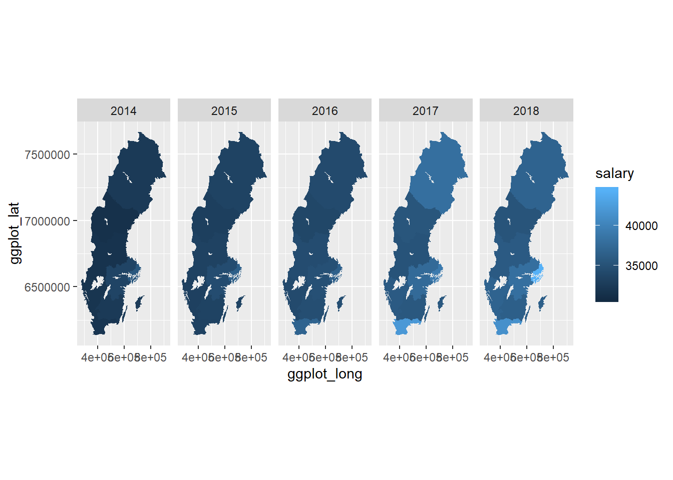
Figure 11: Highest F-value interaction year and region, Nursing professionals
temp <- tb %>%
  filter(`occuptional  (SSYK 2012)` == "541 Other surveillance and security workers")

model <-lm (log(salary) ~ year_n * NUTS2_sh + sex , data = temp)

plot_model(model, type = "pred", terms = c("NUTS2_sh", "year_n"))
## Model has log-transformed response. Back-transforming predictions to original response scale. Standard errors are still on the log-scale.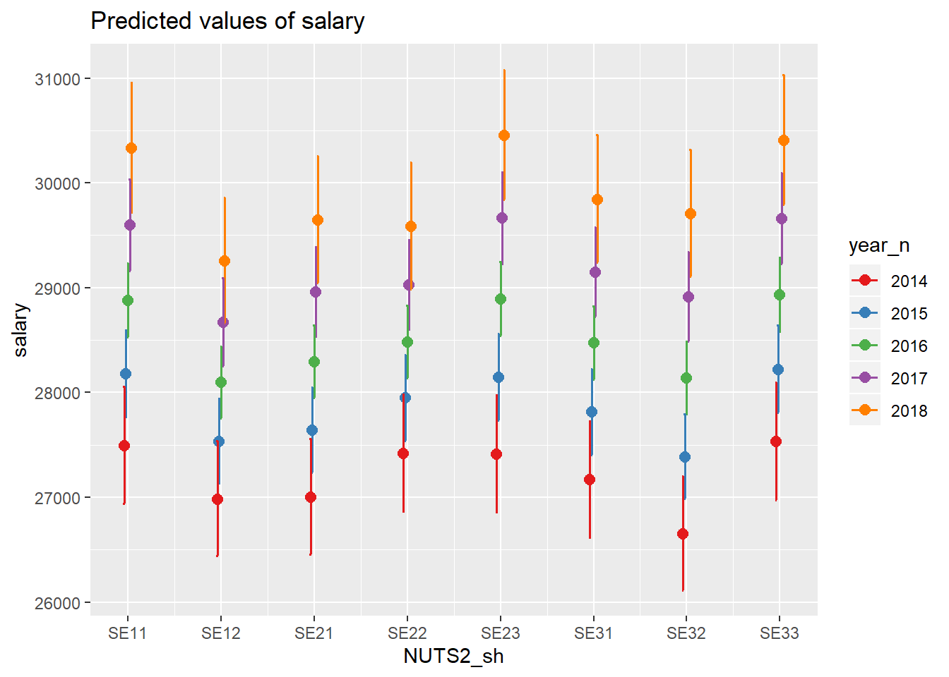
Figure 12: Lowest F-value interaction year and region, Other surveillance and security workers
temp <- tb %>%
  filter(`occuptional  (SSYK 2012)` == "531 Child care workers and teachers aides")

model <-lm (log(salary) ~ year_n * NUTS2_sh * sex , data = temp)

plot_model(model, type = "pred", terms = c("NUTS2_sh", "year_n", "sex"))
## Model has log-transformed response. Back-transforming predictions to original response scale. Standard errors are still on the log-scale.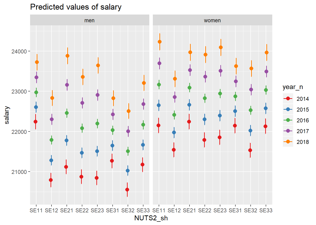
Figure 13: Highest F-value interaction region, year and gender, Child care workers and teachers aides
tb_map %>%
  filter(`occuptional  (SSYK 2012)` == "531 Child care workers and teachers aides") %>%
  filter (sex == "men") %>%
  ggplot() +
    geom_polygon(mapping = aes(x = ggplot_long, y = ggplot_lat, group = lnkod, fill = salary)) +
      facet_grid(. ~ year) +
coord_equal() 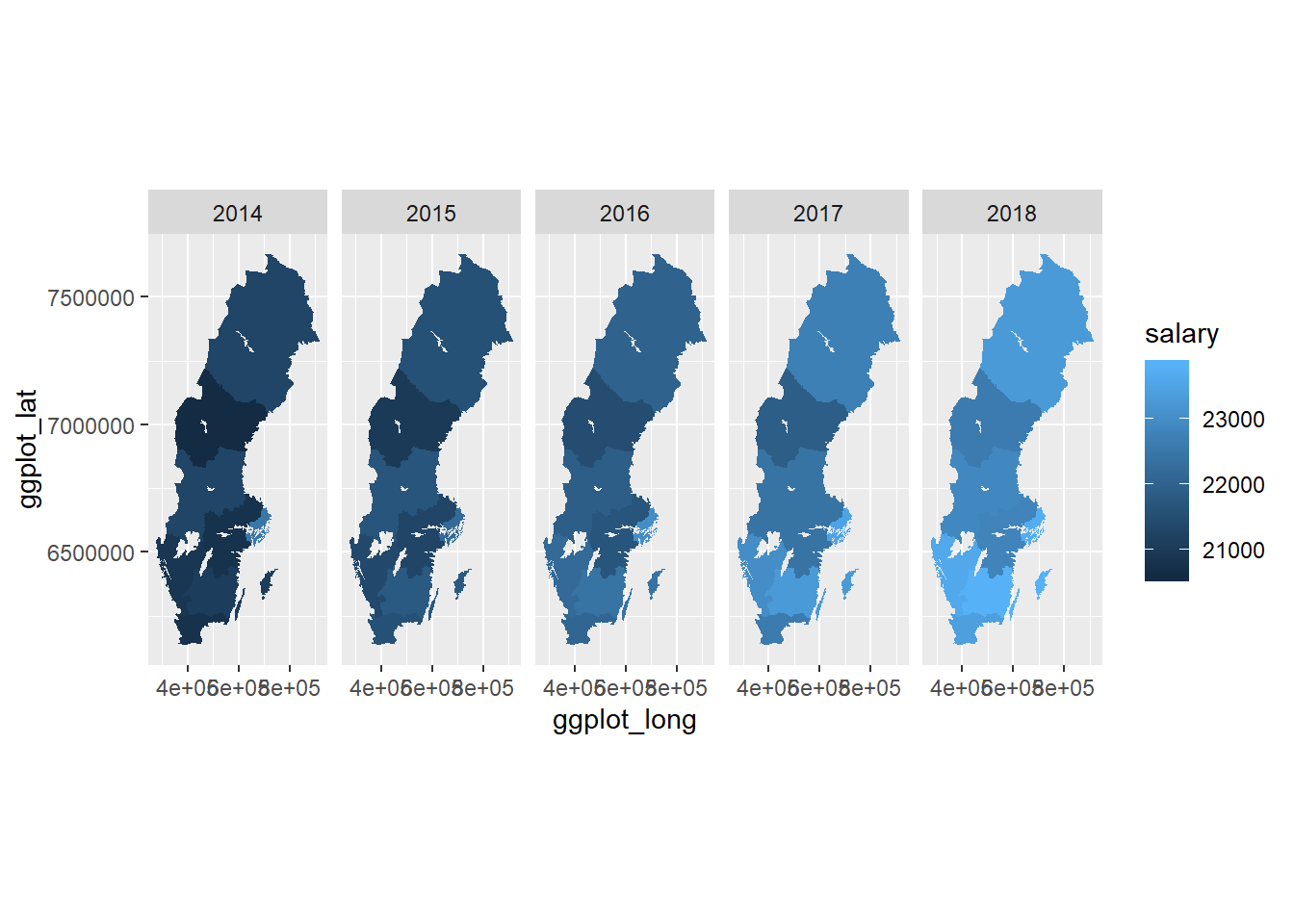
Figure 14: Highest F-value interaction region, year and gender, Child care workers and teachers aides
tb_map %>%
    filter(`occuptional  (SSYK 2012)` == "531 Child care workers and teachers aides") %>%
  filter (sex == "women") %>%
  ggplot() +
    geom_polygon(mapping = aes(x = ggplot_long, y = ggplot_lat, group = lnkod, fill = salary)) +
      facet_grid(. ~ year) +
coord_equal() 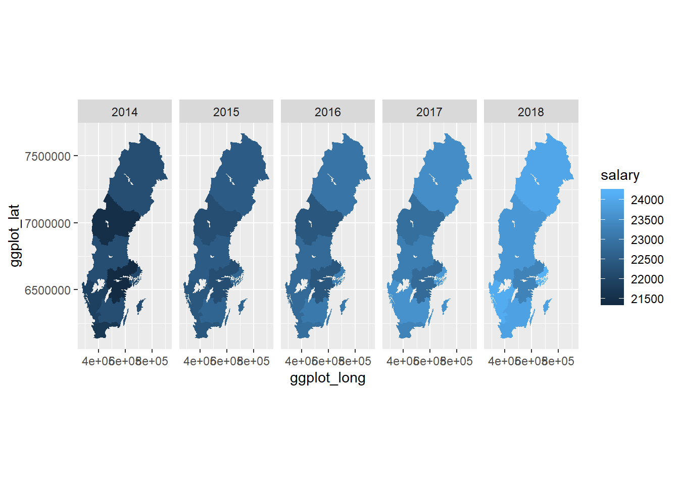
Figure 15: Highest F-value interaction region, year and gender, Child care workers and teachers aides
temp <- tb %>%
  filter(`occuptional  (SSYK 2012)` == "336 Police officers")

model <-lm (log(salary) ~ year_n * NUTS2_sh * sex , data = temp)

plot_model(model, type = "pred", terms = c("NUTS2_sh", "year_n", "sex"))
## Model has log-transformed response. Back-transforming predictions to original response scale. Standard errors are still on the log-scale.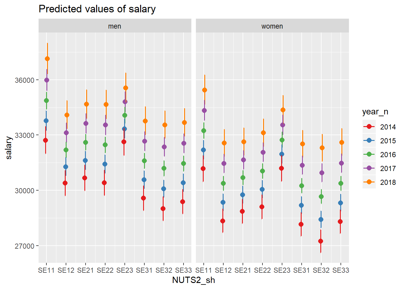
Figure 16: Lowest F-value interaction region, year and gender, Police officers