So far I have analysed the effect of experience, education, gender, year and region on the salary of engineers in Sweden. In this post, I will have a look at the effect of the sector on the salary of engineers in Sweden.
Statistics Sweden use NUTS (Nomenclature des Unités Territoriales Statistiques), which is the EU’s hierarchical regional division, to specify the regions.
First, define libraries and functions.
library (tidyverse) ## -- Attaching packages -------------------------------------- tidyverse 1.3.0 --## v ggplot2 3.2.1 v purrr 0.3.3
## v tibble 2.1.3 v dplyr 0.8.3
## v tidyr 1.0.2 v stringr 1.4.0
## v readr 1.3.1 v forcats 0.4.0## -- Conflicts ----------------------------------------- tidyverse_conflicts() --
## x dplyr::filter() masks stats::filter()
## x dplyr::lag() masks stats::lag()library (broom)
library (car)## Loading required package: carData##
## Attaching package: 'car'## The following object is masked from 'package:dplyr':
##
## recode## The following object is masked from 'package:purrr':
##
## somelibrary (swemaps) # devtools::install_github('reinholdsson/swemaps')
library(sjPlot)## Registered S3 methods overwritten by 'lme4':
## method from
## cooks.distance.influence.merMod car
## influence.merMod car
## dfbeta.influence.merMod car
## dfbetas.influence.merMod car## Install package "strengejacke" from GitHub (`devtools::install_github("strengejacke/strengejacke")`) to load all sj-packages at once!library(leaps)
library(MASS)##
## Attaching package: 'MASS'## The following object is masked from 'package:dplyr':
##
## selectreadfile <- function (file1){
read_csv (file1, col_types = cols(), locale = readr::locale (encoding = "latin1"), na = c("..", "NA")) %>%
gather (starts_with("19"), starts_with("20"), key = "year", value = salary) %>%
drop_na() %>%
mutate (year_n = parse_number (year))
}
nuts <- read.csv("nuts.csv") %>%
mutate(NUTS2_sh = substr(NUTS2, 1, 4))
map_ln_n <- map_ln %>%
mutate(lnkod_n = as.numeric(lnkod)) The data table is downloaded from Statistics Sweden. It is saved as a comma-delimited file without heading, 000000CG.csv, http://www.statistikdatabasen.scb.se/pxweb/en/ssd/.
I have renamed the file to 000000CG_sector.csv because the filename 000000CG.csv was used in a previous post.
The table: Average basic salary, monthly salary and women´s salary as a percentage of men´s salary by region, sector, occupational group (SSYK 2012) and sex. Year 2014 - 2018 Monthly salary 1-3 public sector 4-5 private sector
We expect that the sector is an important factor in salaries. As a null hypothesis, we assume that the sector is not related to the salary and examine if we can reject this hypothesis with the data from Statistics Sweden.
tb <- readfile ("000000CG_sector.csv") %>%
  filter (`occuptional  (SSYK 2012)` == "214 Engineering professionals") %>%
  left_join(nuts %>% distinct (NUTS2_en, NUTS2_sh), by = c("region" = "NUTS2_en"))
## Warning: Column `region`/`NUTS2_en` joining character vector and factor,
## coercing into character vectortb_map <- readfile ("000000CG_sector.csv") %>%
filter (`occuptional (SSYK 2012)` == "214 Engineering professionals") %>%
left_join(nuts, by = c("region" = "NUTS2_en")) ## Warning: Column `region`/`NUTS2_en` joining character vector and factor,
## coercing into character vectortb_map %>%
filter (sector == "1-3 public sector") %>%
right_join(map_ln_n, by = c("Länskod" = "lnkod_n")) %>%
ggplot() +
geom_polygon(mapping = aes(x = ggplot_long, y = ggplot_lat, group = lnkod, fill = salary)) +
facet_grid(. ~ year) +
coord_equal() 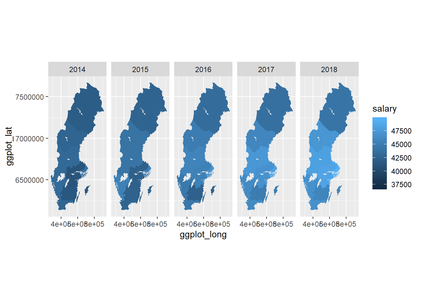
Figure 1: SSYK 214, Architects, engineers and related professionals, public sector, Year 2014 - 2018
tb_map %>%
  filter (sector == "4-5 private sector") %>%
  right_join(map_ln_n, by = c("Länskod" = "lnkod_n")) %>%
  ggplot() +
    geom_polygon(mapping = aes(x = ggplot_long, y = ggplot_lat, group = lnkod, fill = salary)) +
    facet_grid(. ~ year) +
coord_equal() 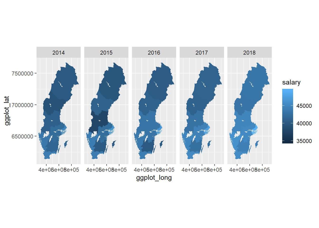
Figure 2: SSYK 214, Architects, engineers and related professionals, private sector, Year 2014 - 2018
tb %>%
  ggplot () +
    geom_point (mapping = aes(x = year_n, y = salary, colour = region, shape=sex)) +
    facet_grid(. ~ sector) +
  labs(
    x = "Year",
    y = "Salary (SEK/month)"
  )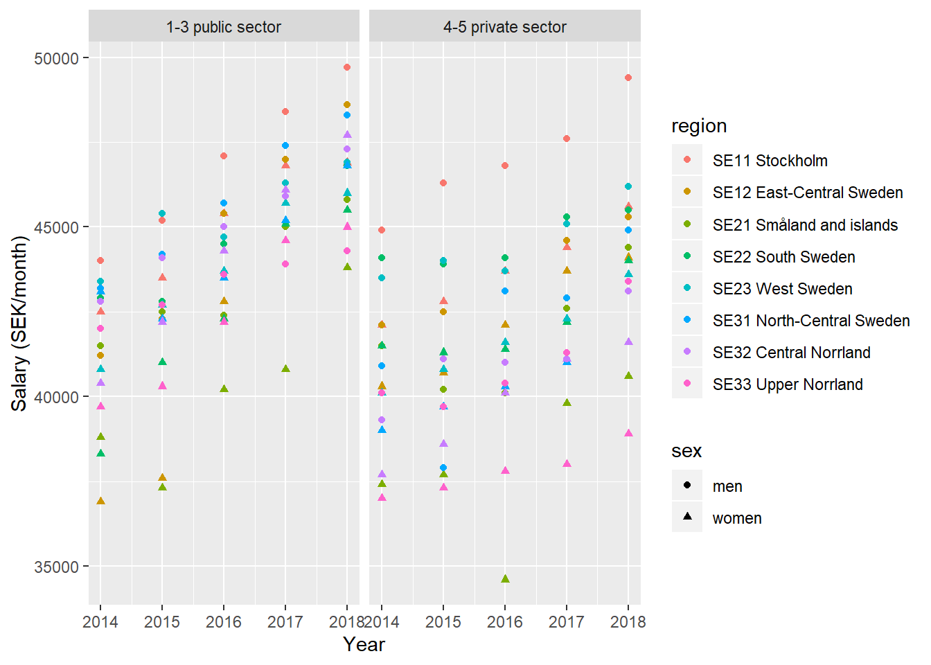
Figure 3: SSYK 214, Architects, engineers and related professionals, Year 2014 - 2018
Before I investigate all possible combinations of the sector and the other factors I shall see if there is some way to predict what factors and interactions that are most significant.
First, use regsubsets to find the model which minimises AIC (Akaike information criterion). Regsubsets is a generic function for regression subset selection with methods for formula and matrix arguments.
b <- regsubsets (log(salary) ~ sector * (year_n + sex + NUTS2_sh), data = tb,  nvmax = 20)
rs <- summary(b)
AIC <- 50 * log (rs$rss / 50) + (2:20) * 2
which.min (AIC)
## [1] 13names (rs$which[13,])[rs$which[13,]]## [1] "(Intercept)"
## [2] "sector4-5 private sector"
## [3] "year_n"
## [4] "sexwomen"
## [5] "NUTS2_shSE12"
## [6] "NUTS2_shSE21"
## [7] "NUTS2_shSE22"
## [8] "NUTS2_shSE33"
## [9] "sector4-5 private sector:year_n"
## [10] "sector4-5 private sector:NUTS2_shSE21"
## [11] "sector4-5 private sector:NUTS2_shSE23"
## [12] "sector4-5 private sector:NUTS2_shSE31"
## [13] "sector4-5 private sector:NUTS2_shSE32"
## [14] "sector4-5 private sector:NUTS2_shSE33"As a complement, I use stepwise model selection to find the model which fits the data best. StepAIC performs stepwise model selection by AIC.
model <-lm (log(salary) ~ year_n * sex * NUTS2_sh * sector, data = tb)
b <- stepAIC(model, direction = c("both"))
## Start: AIC=-1200.79
## log(salary) ~ year_n * sex * NUTS2_sh * sector
##
## Df Sum of Sq RSS AIC
## - year_n:sex:NUTS2_sh:sector 7 0.001441 0.041008 -1209.1
## <none> 0.039567 -1200.8
##
## Step: AIC=-1209.07
## log(salary) ~ year_n + sex + NUTS2_sh + sector + year_n:sex +
## year_n:NUTS2_sh + sex:NUTS2_sh + year_n:sector + sex:sector +
## NUTS2_sh:sector + year_n:sex:NUTS2_sh + year_n:sex:sector +
## year_n:NUTS2_sh:sector + sex:NUTS2_sh:sector
##
## Df Sum of Sq RSS AIC
## <none> 0.041008 -1209.1
## - year_n:sex:NUTS2_sh 7 0.0047401 0.045748 -1205.6
## - year_n:sex:sector 1 0.0022478 0.043256 -1202.5
## - year_n:NUTS2_sh:sector 7 0.0058131 0.046821 -1201.9
## + year_n:sex:NUTS2_sh:sector 7 0.0014410 0.039567 -1200.8
## - sex:NUTS2_sh:sector 7 0.0080176 0.049026 -1194.5model <- lm(log(salary) ~ year_n + sex + NUTS2_sh + sector +
year_n:sex + year_n:NUTS2_sh + sex:NUTS2_sh + year_n:sector +
sex:sector + NUTS2_sh:sector + year_n:sex:NUTS2_sh + year_n:sex:sector +
year_n:NUTS2_sh:sector + sex:NUTS2_sh:sector, data = tb)
summary(model)$adj.r.squared ## [1] 0.9135882Anova(model, type = 2) %>%
tidy() %>%
arrange (desc (statistic)) %>%
filter(p.value < 0.05) %>%
knitr::kable(
booktabs = TRUE,
caption = 'Anova report from linear model fit')| term | sumsq | df | statistic | p.value |
|---|---|---|---|---|
| year_n | 0.2069351 | 1 | 519.760278 | 0.0000000 |
| sex | 0.1113983 | 2 | 139.899908 | 0.0000000 |
| sector | 0.0952663 | 2 | 119.640560 | 0.0000000 |
| NUTS2_sh | 0.2322097 | 14 | 41.660196 | 0.0000000 |
| year_n:sector | 0.0120669 | 1 | 30.308411 | 0.0000003 |
| NUTS2_sh:sector | 0.0523275 | 7 | 18.775900 | 0.0000000 |
| year_n:sex | 0.0023493 | 1 | 5.900761 | 0.0168659 |
| year_n:sex:sector | 0.0022478 | 1 | 5.645699 | 0.0193467 |
| sex:sector | 0.0018231 | 1 | 4.579079 | 0.0347260 |
| sex:NUTS2_sh | 0.0106289 | 7 | 3.813803 | 0.0010092 |
| sex:NUTS2_sh:sector | 0.0080176 | 7 | 2.876825 | 0.0087375 |
| year_n:NUTS2_sh | 0.0078670 | 7 | 2.822810 | 0.0098854 |
There are interactions between the different factors that are significant, i.e. have a p-value less than 0,05 but does not qualify because it´s inclusion in the model does not imply that it lowers the AIC value. The tradeoff between the goodness of fit of the model and the simplicity of the model leads me to exclude those interactions from the model we will examine further.
The model I chose from based on the AIC results is: log(salary) ~ year_n * sector + NUTS2_sh * sector + sex
From this model, the F-value from the Anova table for the sector is 146 (Pr(>F) < 2.2e-16), sufficient for rejecting the null hypothesis that the sector has no effect on the salary holding year as constant. The adjusted R-squared value is 0,870 implying a good fit of the model.
model <- model <-lm (log(salary) ~ year_n * sector + NUTS2_sh * sector + sex, data = tb)
tb <- bind_cols(tb, as_tibble(exp(predict(model, tb, interval = "confidence"))))
tb %>%
  ggplot () +
    geom_point (mapping = aes(x = year_n,y = fit, colour = region, shape=sex)) +
    facet_grid(. ~ sector) +
  labs(
    x = "Year",
    y = "Salary (SEK/month)"
  )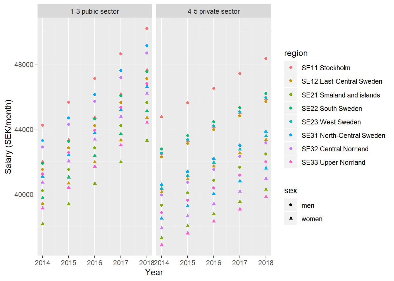
Figure 4: Model fit, SSYK 214, Architects, engineers and related professionals, Year 2014 - 2018
summary(model) %>%
  tidy() %>%
  knitr::kable(
  booktabs = TRUE,
caption = 'Summary from linear model fit')| term | estimate | std.error | statistic | p.value |
|---|---|---|---|---|
| (Intercept) | -52.8857464 | 3.9015473 | -13.5550700 | 0.0000000 |
| year_n | 0.0315705 | 0.0019353 | 16.3130867 | 0.0000000 |
| sector4-5 private sector | 24.7466021 | 5.5176204 | 4.4850135 | 0.0000150 |
| NUTS2_shSE12 | -0.0633886 | 0.0109476 | -5.7901587 | 0.0000000 |
| NUTS2_shSE21 | -0.0951854 | 0.0109476 | -8.6946021 | 0.0000000 |
| NUTS2_shSE22 | -0.0542415 | 0.0109476 | -4.9546264 | 0.0000020 |
| NUTS2_shSE23 | -0.0304669 | 0.0109476 | -2.7829655 | 0.0061252 |
| NUTS2_shSE31 | -0.0213974 | 0.0109476 | -1.9545201 | 0.0526182 |
| NUTS2_shSE32 | -0.0304128 | 0.0109476 | -2.7780207 | 0.0062142 |
| NUTS2_shSE33 | -0.0700399 | 0.0109476 | -6.3977139 | 0.0000000 |
| sexwomen | -0.0523393 | 0.0038706 | -13.5223569 | 0.0000000 |
| year_n:sector4-5 private sector | -0.0122815 | 0.0027369 | -4.4873679 | 0.0000149 |
| sector4-5 private sector:NUTS2_shSE12 | 0.0069109 | 0.0154823 | 0.4463758 | 0.6560106 |
| sector4-5 private sector:NUTS2_shSE21 | -0.0344624 | 0.0154823 | -2.2259214 | 0.0276066 |
| sector4-5 private sector:NUTS2_shSE22 | 0.0089387 | 0.0154823 | 0.5773509 | 0.5646232 |
| sector4-5 private sector:NUTS2_shSE23 | -0.0206495 | 0.0154823 | -1.3337474 | 0.1844371 |
| sector4-5 private sector:NUTS2_shSE31 | -0.0765503 | 0.0154823 | -4.9443769 | 0.0000021 |
| sector4-5 private sector:NUTS2_shSE32 | -0.0832467 | 0.0154823 | -5.3768944 | 0.0000003 |
| sector4-5 private sector:NUTS2_shSE33 | -0.0711249 | 0.0154823 | -4.5939480 | 0.0000096 |
summary(model)$adj.r.squared ## [1] 0.8699372Anova(model, type=2) %>%
tidy() %>%
knitr::kable(
booktabs = TRUE,
caption = 'Anova report from linear model fit')| term | sumsq | df | statistic | p.value |
|---|---|---|---|---|
| year_n | 0.2069351 | 1 | 345.32122 | 0.00e+00 |
| sector | 0.0872899 | 1 | 145.66429 | 0.00e+00 |
| NUTS2_sh | 0.1798897 | 7 | 42.88421 | 0.00e+00 |
| sex | 0.1095761 | 1 | 182.85414 | 0.00e+00 |
| year_n:sector | 0.0120669 | 1 | 20.13647 | 1.49e-05 |
| sector:NUTS2_sh | 0.0523275 | 7 | 12.47444 | 0.00e+00 |
| Residuals | 0.0844948 | 141 | NA | NA |
plot(model, which = 1)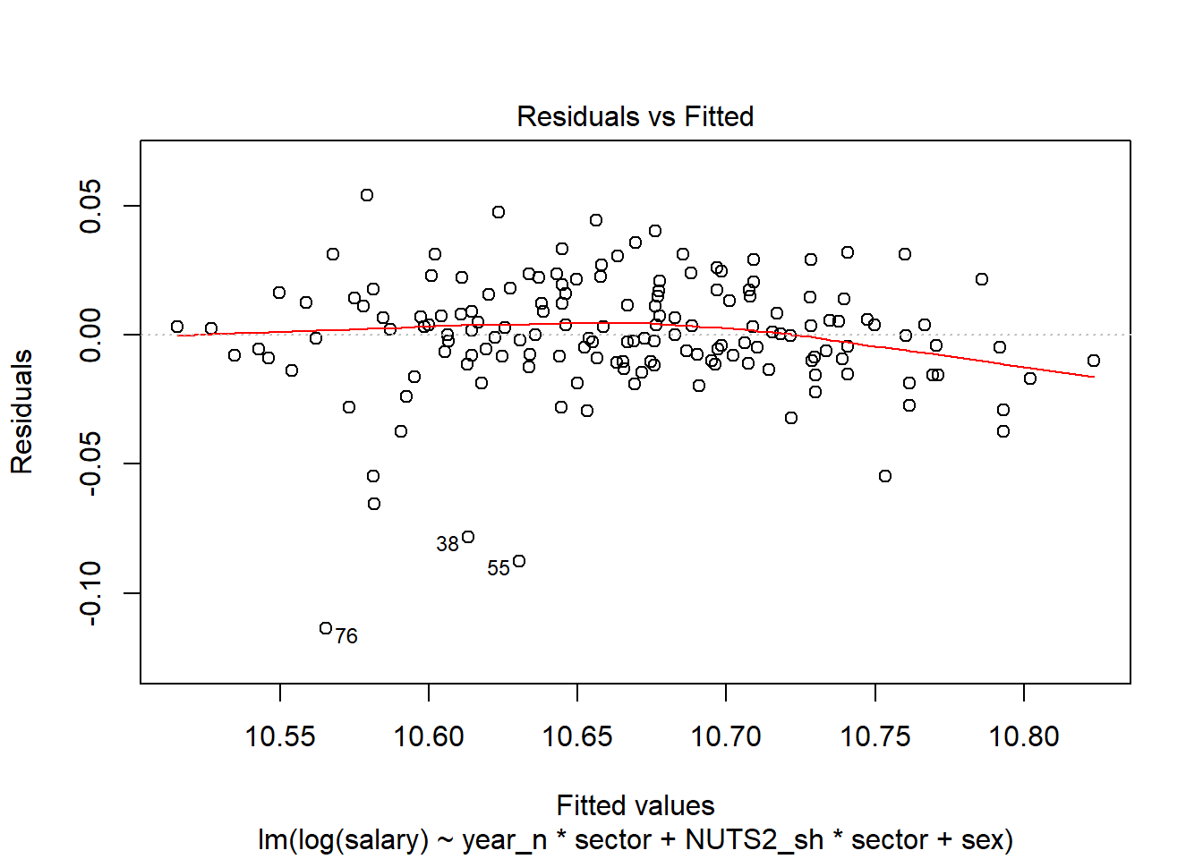
Figure 5: Model fit, SSYK 214, Architects, engineers and related professionals, Year 2014 - 2018
tb[38,]## # A tibble: 1 x 11
## region sector `occuptional (~ sex year salary year_n NUTS2_sh fit
## <chr> <chr> <chr> <chr> <chr> <dbl> <dbl> <chr> <dbl>
## 1 SE12 ~ 1-3 p~ 214 Engineering~ women 2015 37600 2015 SE12 40664.
## # ... with 2 more variables: lwr <dbl>, upr <dbl>tb[55,]## # A tibble: 1 x 11
## region sector `occuptional (~ sex year salary year_n NUTS2_sh fit
## <chr> <chr> <chr> <chr> <chr> <dbl> <dbl> <chr> <dbl>
## 1 SE31 ~ 4-5 p~ 214 Engineering~ men 2015 37900 2015 SE31 41366.
## # ... with 2 more variables: lwr <dbl>, upr <dbl>tb[76,]## # A tibble: 1 x 11
## region sector `occuptional (~ sex year salary year_n NUTS2_sh fit
## <chr> <chr> <chr> <chr> <chr> <dbl> <dbl> <chr> <dbl>
## 1 SE21 ~ 4-5 p~ 214 Engineering~ women 2016 34600 2016 SE21 38773.
## # ... with 2 more variables: lwr <dbl>, upr <dbl>Let’s check what we have found.
For the sake of comparison, a model with no interactions.
model <-lm (log(salary) ~ year_n + sex + NUTS2_sh + sector, data = tb)

plot_model(model, type = "pred", terms = c("NUTS2_sh", "year_n", "sex", "sector"))
## Model has log-transformed response. Back-transforming predictions to original response scale. Standard errors are still on the log-scale.## Warning: Package `see` needed to plot multiple panels in one integrated figure.
## Please install it by typing `install.packages("see", dependencies = TRUE)` into
## the console.## [[1]]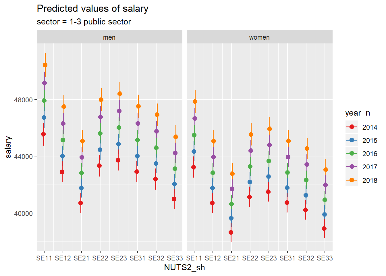
Figure 6: SSYK 214, Architects, engineers and related professionals, Year 2014 - 2018
##
## [[2]]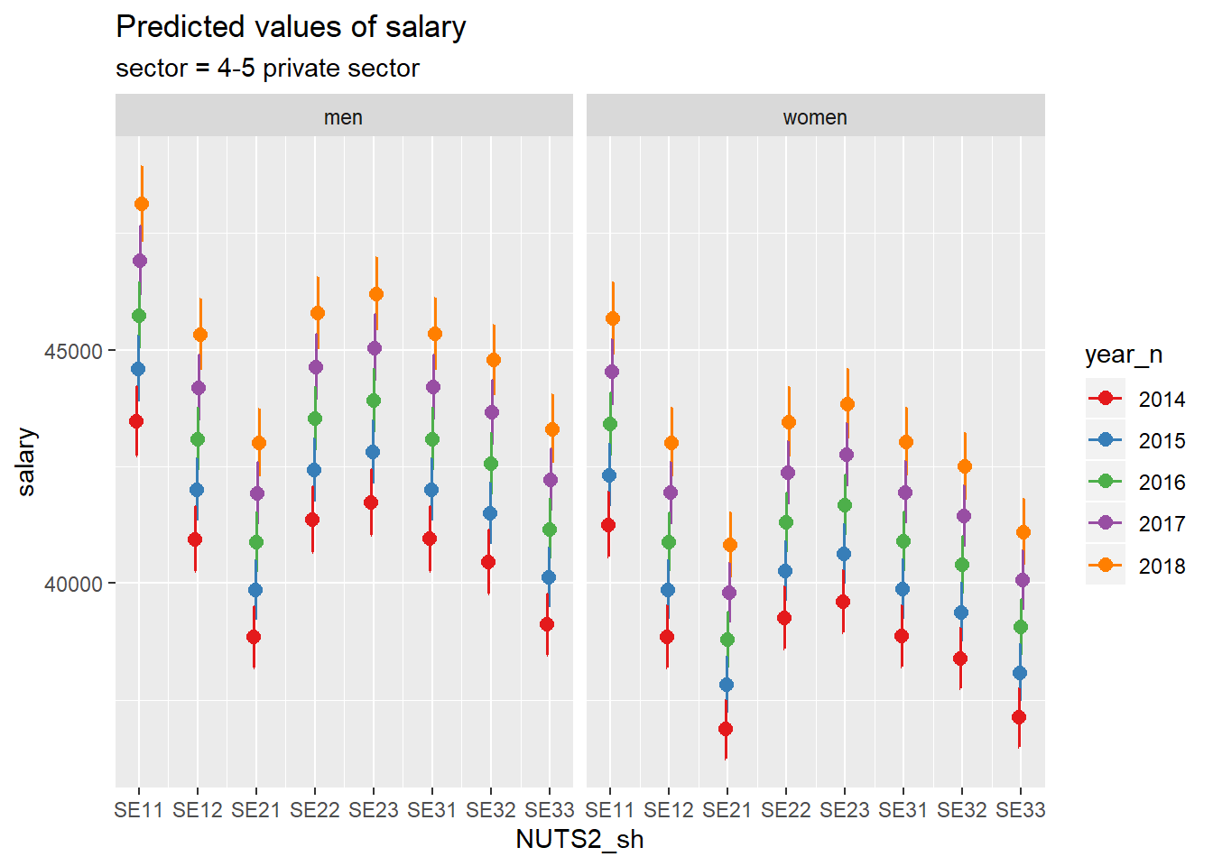
Figure 7: SSYK 214, Architects, engineers and related professionals, Year 2014 - 2018
First, we investigate the interaction between region and sector. All plots below are done with the model which minimised the AIC.
model <- model <-lm (log(salary) ~ year_n * sector + NUTS2_sh * sector + sex, data = tb)

plot_model(model, type = "pred", terms = c("NUTS2_sh", "sector"))
## Model has log-transformed response. Back-transforming predictions to original response scale. Standard errors are still on the log-scale.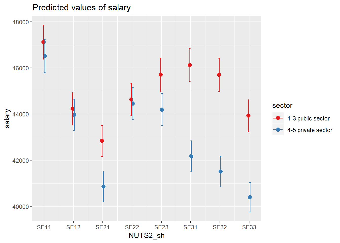
Figure 8: SSYK 214, Architects, engineers and related professionals, Year 2014 - 2018
Also, examine the relationship between gender and sector.
model <- model <-lm (log(salary) ~ year_n * sector + NUTS2_sh * sector + sex, data = tb)

plot_model(model, type = "pred", terms = c("sector", "sex"))
## Model has log-transformed response. Back-transforming predictions to original response scale. Standard errors are still on the log-scale.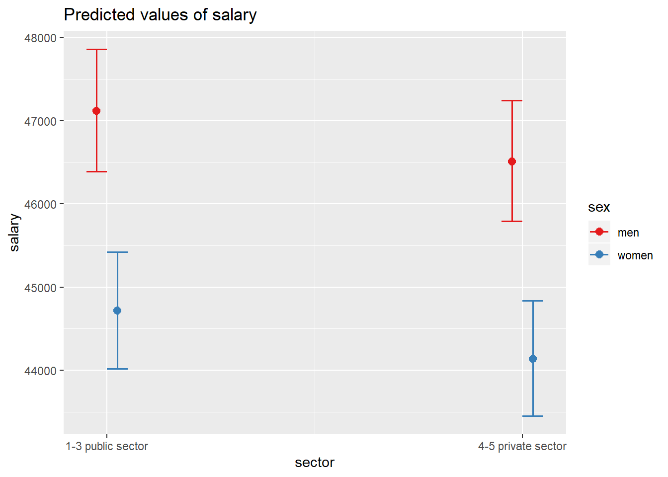
Figure 9: SSYK 214, Architects, engineers and related professionals, Year 2014 - 2018
And the interaction between year and sector.
model <- model <-lm (log(salary) ~ year_n * sector + NUTS2_sh * sector + sex, data = tb)

plot_model(model, type = "pred", terms = c("year_n", "sector"))
## Model has log-transformed response. Back-transforming predictions to original response scale. Standard errors are still on the log-scale.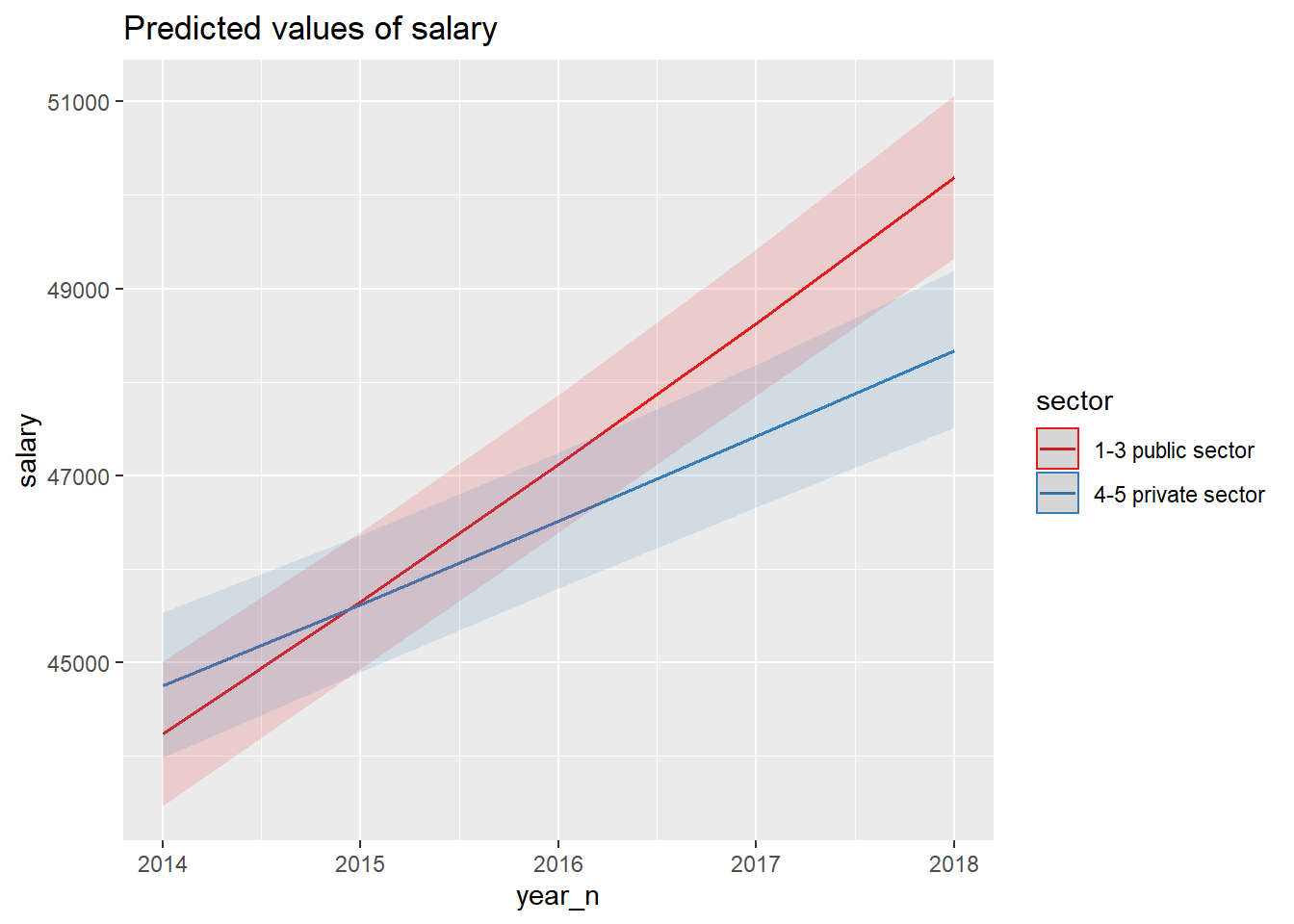
Figure 10: SSYK 214, Architects, engineers and related professionals, Year 2014 - 2018
The relationship between gender, sector and region.
model <- model <-lm (log(salary) ~ year_n * sector + NUTS2_sh * sector + sex, data = tb)

plot_model(model, type = "pred", terms = c("NUTS2_sh", "sector", "sex"))
## Model has log-transformed response. Back-transforming predictions to original response scale. Standard errors are still on the log-scale.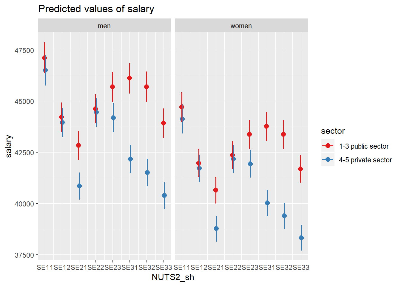
Figure 11: SSYK 214, Architects, engineers and related professionals, Year 2014 - 2018
The relationship between gender, sector and year.
model <- model <-lm (log(salary) ~ year_n * sector + NUTS2_sh * sector + sex, data = tb)

plot_model(model, type = "pred", terms = c("year_n", "sector", "sex"))
## Model has log-transformed response. Back-transforming predictions to original response scale. Standard errors are still on the log-scale.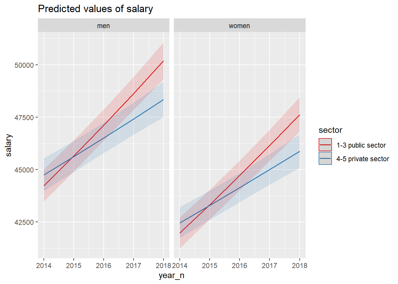
Figure 12: SSYK 214, Architects, engineers and related professionals, Year 2014 - 2018
The relationship between region, sector and year.
model <- model <-lm (log(salary) ~ year_n * sector + NUTS2_sh * sector + sex, data = tb)

plot_model(model, type = "pred", terms = c("NUTS2_sh", "year_n", "sector"))
## Model has log-transformed response. Back-transforming predictions to original response scale. Standard errors are still on the log-scale.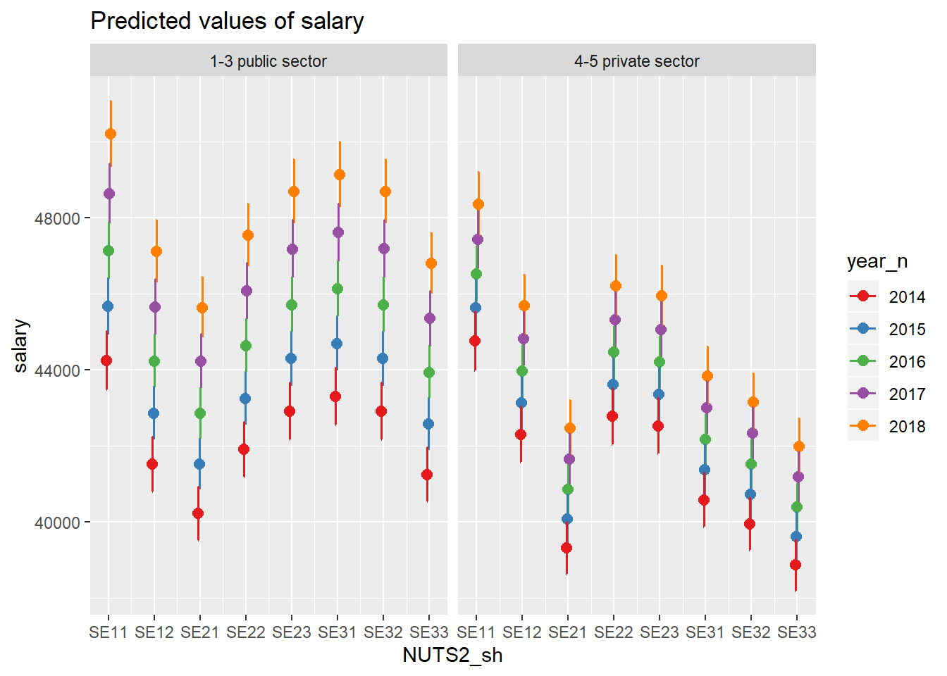
Figure 13: SSYK 214, Architects, engineers and related professionals, Year 2014 - 2018
The relationship between gender, region, sector and year.
model <- model <-lm (log(salary) ~ year_n * sector + NUTS2_sh * sector + sex, data = tb)

plot_model(model, type = "pred", terms = c("NUTS2_sh", "year_n", "sector", "sex"))
## Model has log-transformed response. Back-transforming predictions to original response scale. Standard errors are still on the log-scale.## Warning: Package `see` needed to plot multiple panels in one integrated figure.
## Please install it by typing `install.packages("see", dependencies = TRUE)` into
## the console.## [[1]]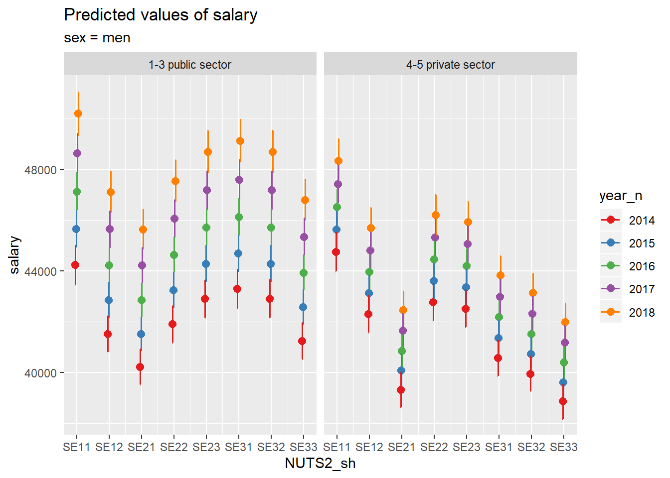
Figure 14: SSYK 214, Architects, engineers and related professionals, Year 2014 - 2018
##
## [[2]]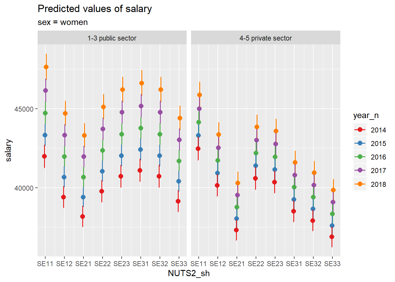
Figure 15: SSYK 214, Architects, engineers and related professionals, Year 2014 - 2018