To complete the analysis on the significance of the sector on the salary for different occupational groups in Sweden I will in this post examine the correlation between salary and sector using statistics for education.
The F-value from the Anova table is used as the single value to discriminate how much the region and salary correlates. For exploratory analysis, the Anova value seems good enough.
First, define libraries and functions.
library (tidyverse)## -- Attaching packages --------------------------------------------------- tidyverse 1.3.0 --## v ggplot2 3.2.1 v purrr 0.3.3
## v tibble 2.1.3 v dplyr 0.8.3
## v tidyr 1.0.2 v stringr 1.4.0
## v readr 1.3.1 v forcats 0.4.0## -- Conflicts ------------------------------------------------------ tidyverse_conflicts() --
## x dplyr::filter() masks stats::filter()
## x dplyr::lag() masks stats::lag()library (broom)
library (car)## Loading required package: carData##
## Attaching package: 'car'## The following object is masked from 'package:dplyr':
##
## recode## The following object is masked from 'package:purrr':
##
## somelibrary (sjPlot)## Registered S3 methods overwritten by 'lme4':
## method from
## cooks.distance.influence.merMod car
## influence.merMod car
## dfbeta.influence.merMod car
## dfbetas.influence.merMod car## Learn more about sjPlot with 'browseVignettes("sjPlot")'.readfile <- function (file1){read_csv (file1, col_types = cols(), locale = readr::locale (encoding = "latin1"), na = c("..", "NA")) %>%
gather (starts_with("19"), starts_with("20"), key = "year", value = salary) %>%
drop_na() %>%
mutate (year_n = parse_number (year))
}The data table is downloaded from Statistics Sweden. It is saved as a comma-delimited file without heading, 000000CY.csv, http://www.statistikdatabasen.scb.se/pxweb/en/ssd/.
I have renamed the file to 000000CY_sector.csv because the filename 000000CY.csv was used in a previous post.
The table: Average basic salary, monthly salary and women´s salary as a percentage of men´s salary by sector, occupational group (SSYK 2012), sex and educational level (SUN). Year 2014 - 2018 Monthly salary 1-3 public sector 4-5 private sector
In the plot and tables, you can also find information on how the increase in salaries per year for each occupational group is affected when the interactions are taken into account.
tb <- readfile("000000CY_sector.csv") %>%
  mutate(edulevel = `level of education`)

numedulevel <- read.csv("edulevel.csv")

numedulevel %>%
  knitr::kable(
  booktabs = TRUE,
caption = 'Initial approach, length of education') | level.of.education | eduyears |
|---|---|
| primary and secondary education 9-10 years (ISCED97 2) | 9 |
| upper secondary education, 2 years or less (ISCED97 3C) | 11 |
| upper secondary education 3 years (ISCED97 3A) | 12 |
| post-secondary education, less than 3 years (ISCED97 4+5B) | 14 |
| post-secondary education 3 years or more (ISCED97 5A) | 15 |
| post-graduate education (ISCED97 6) | 19 |
| no information about level of educational attainment | NA |
tbnum <- tb %>%
  right_join(numedulevel, by = c("level of education" = "level.of.education")) %>%
  filter(!is.na(eduyears)) %>%
  mutate(eduyears = factor(eduyears))
## Warning: Column `level of education`/`level.of.education` joining character
## vector and factor, coercing into character vectorsummary_table = vector()
anova_table = vector()
for (i in unique(tbnum$`occuptional (SSYK 2012)`)){
temp <- filter(tbnum, `occuptional (SSYK 2012)` == i)
if (dim(temp)[1] > 90){
model <- lm(log(salary) ~ edulevel + sex + year_n + sector, data = temp)
summary_table <- rbind (summary_table, mutate (tidy (summary (model)), ssyk = i, interaction = "none"))
anova_table <- rbind (anova_table, mutate (tidy (Anova (model, type = 2)), ssyk = i, interaction = "none"))
model <- lm(log(salary) ~ edulevel * sector + sex + year_n, data = temp)
summary_table <- rbind (summary_table, mutate (tidy (summary (model)), ssyk = i, interaction = "sector and edulevel"))
anova_table <- rbind (anova_table, mutate (tidy (Anova (model, type = 2)), ssyk = i, interaction = "sector and edulevel"))
model <- lm(log(salary) ~ edulevel + sector * sex + year_n, data = temp)
summary_table <- rbind (summary_table, mutate (tidy (summary (model)), ssyk = i, interaction = "sector and sex"))
anova_table <- rbind (anova_table, mutate (tidy (Anova (model, type = 2)), ssyk = i, interaction = "sector and sex"))
model <- lm(log(salary) ~ edulevel + year_n * sector + sex, data = temp)
summary_table <- rbind (summary_table, mutate (tidy (summary (model)), ssyk = i, interaction = "sector and year"))
anova_table <- rbind (anova_table, mutate (tidy (Anova (model, type = 2)), ssyk = i, interaction = "sector and year"))
model <- lm(log(salary) ~ edulevel * sector * sex * year_n, data = temp)
summary_table <- rbind (summary_table, mutate (tidy (summary (model)), ssyk = i, interaction = "sector, year, edulevel and sex"))
anova_table <- rbind (anova_table, mutate (tidy (Anova (model, type = 2)), ssyk = i, interaction = "sector, year, edulevel and sex"))
}
}## Note: model has aliased coefficients
## sums of squares computed by model comparison
## Note: model has aliased coefficients
## sums of squares computed by model comparison
## Note: model has aliased coefficients
## sums of squares computed by model comparison
## Note: model has aliased coefficients
## sums of squares computed by model comparison
## Note: model has aliased coefficients
## sums of squares computed by model comparison
## Note: model has aliased coefficients
## sums of squares computed by model comparison
## Note: model has aliased coefficients
## sums of squares computed by model comparison
## Note: model has aliased coefficients
## sums of squares computed by model comparison
## Note: model has aliased coefficients
## sums of squares computed by model comparison
## Note: model has aliased coefficients
## sums of squares computed by model comparison
## Note: model has aliased coefficients
## sums of squares computed by model comparison
## Note: model has aliased coefficients
## sums of squares computed by model comparison
## Note: model has aliased coefficients
## sums of squares computed by model comparison
## Note: model has aliased coefficients
## sums of squares computed by model comparison
## Note: model has aliased coefficients
## sums of squares computed by model comparison
## Note: model has aliased coefficients
## sums of squares computed by model comparison
## Note: model has aliased coefficients
## sums of squares computed by model comparison
## Note: model has aliased coefficients
## sums of squares computed by model comparison
## Note: model has aliased coefficients
## sums of squares computed by model comparison
## Note: model has aliased coefficients
## sums of squares computed by model comparison
## Note: model has aliased coefficients
## sums of squares computed by model comparison
## Note: model has aliased coefficients
## sums of squares computed by model comparison
## Note: model has aliased coefficients
## sums of squares computed by model comparison
## Note: model has aliased coefficients
## sums of squares computed by model comparison
## Note: model has aliased coefficients
## sums of squares computed by model comparison
## Note: model has aliased coefficients
## sums of squares computed by model comparison
## Note: model has aliased coefficients
## sums of squares computed by model comparison
## Note: model has aliased coefficients
## sums of squares computed by model comparison
## Note: model has aliased coefficients
## sums of squares computed by model comparison
## Note: model has aliased coefficients
## sums of squares computed by model comparison
## Note: model has aliased coefficients
## sums of squares computed by model comparison
## Note: model has aliased coefficients
## sums of squares computed by model comparison
## Note: model has aliased coefficients
## sums of squares computed by model comparison
## Note: model has aliased coefficients
## sums of squares computed by model comparison
## Note: model has aliased coefficients
## sums of squares computed by model comparison
## Note: model has aliased coefficients
## sums of squares computed by model comparison
## Note: model has aliased coefficients
## sums of squares computed by model comparison
## Note: model has aliased coefficients
## sums of squares computed by model comparison
## Note: model has aliased coefficients
## sums of squares computed by model comparison
## Note: model has aliased coefficients
## sums of squares computed by model comparison
## Note: model has aliased coefficients
## sums of squares computed by model comparison
## Note: model has aliased coefficients
## sums of squares computed by model comparison
## Note: model has aliased coefficients
## sums of squares computed by model comparison
## Note: model has aliased coefficients
## sums of squares computed by model comparison
## Note: model has aliased coefficients
## sums of squares computed by model comparison
## Note: model has aliased coefficients
## sums of squares computed by model comparison
## Note: model has aliased coefficients
## sums of squares computed by model comparison
## Note: model has aliased coefficients
## sums of squares computed by model comparison
## Note: model has aliased coefficients
## sums of squares computed by model comparison
## Note: model has aliased coefficients
## sums of squares computed by model comparison
## Note: model has aliased coefficients
## sums of squares computed by model comparison
## Note: model has aliased coefficients
## sums of squares computed by model comparison
## Note: model has aliased coefficients
## sums of squares computed by model comparison
## Note: model has aliased coefficients
## sums of squares computed by model comparison
## Note: model has aliased coefficients
## sums of squares computed by model comparison
## Note: model has aliased coefficients
## sums of squares computed by model comparison
## Note: model has aliased coefficients
## sums of squares computed by model comparison
## Note: model has aliased coefficients
## sums of squares computed by model comparison
## Note: model has aliased coefficients
## sums of squares computed by model comparison
## Note: model has aliased coefficients
## sums of squares computed by model comparison
## Note: model has aliased coefficients
## sums of squares computed by model comparison
## Note: model has aliased coefficients
## sums of squares computed by model comparison
## Note: model has aliased coefficients
## sums of squares computed by model comparisonanova_table <- anova_table %>% rowwise() %>% mutate(contcol = str_count(term, ":"))
summary_table <- summary_table %>% rowwise() %>% mutate(contcol = str_count(term, ":"))
merge(summary_table, anova_table, by = c("ssyk", "interaction"), all = TRUE) %>%
filter (term.x == "year_n") %>%
filter (term.y == "sector") %>%
filter (interaction == "none") %>%
mutate (estimate = (exp(estimate) - 1) * 100) %>%
ggplot () +
geom_point (mapping = aes(x = estimate, y = statistic.y, colour = interaction)) +
labs(
x = "Increase in salaries (% / year)",
y = "F-value for sector"
) 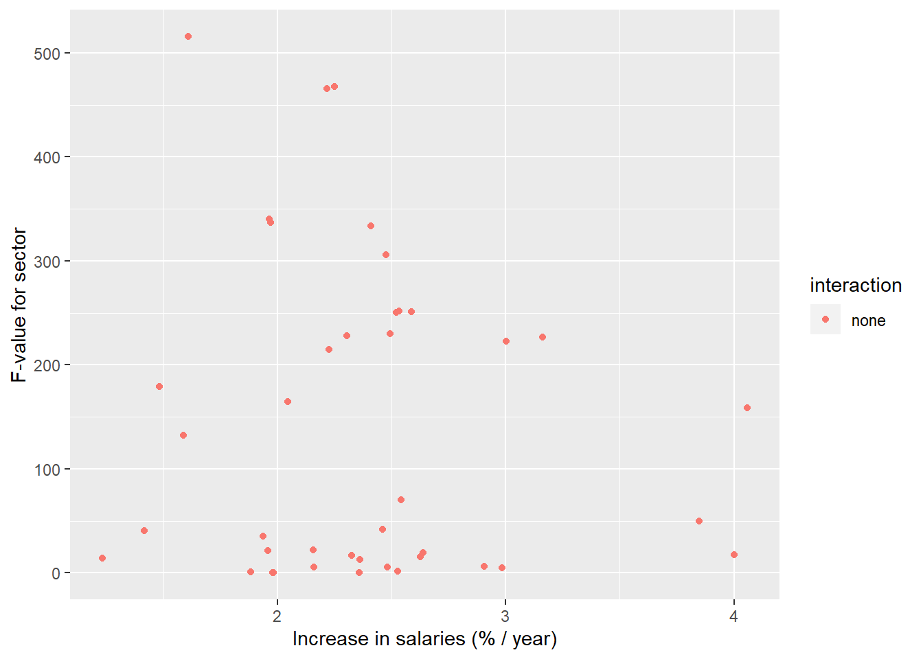
Figure 1: The significance of the sector on the salary in Sweden, a comparison between different occupational groups, Year 2014 - 2018
merge(summary_table, anova_table, by = c("ssyk", "interaction"), all = TRUE) %>%
  filter (term.x == "year_n") %>%
  filter (contcol.y > 0) %>%
  # only look at the interactions between all four variables in the case with interaction sector, year, edulevel and sex
  filter (!(contcol.y < 3 & interaction == "sector, year, edulevel and sex")) %>%

  mutate (estimate = (exp(estimate) - 1) * 100) %>%
  ggplot () +
    geom_point (mapping = aes(x = estimate, y = statistic.y, colour = interaction)) +
    labs(
      x = "Increase in salaries (% / year)",
      y = "F-value for interaction"
) 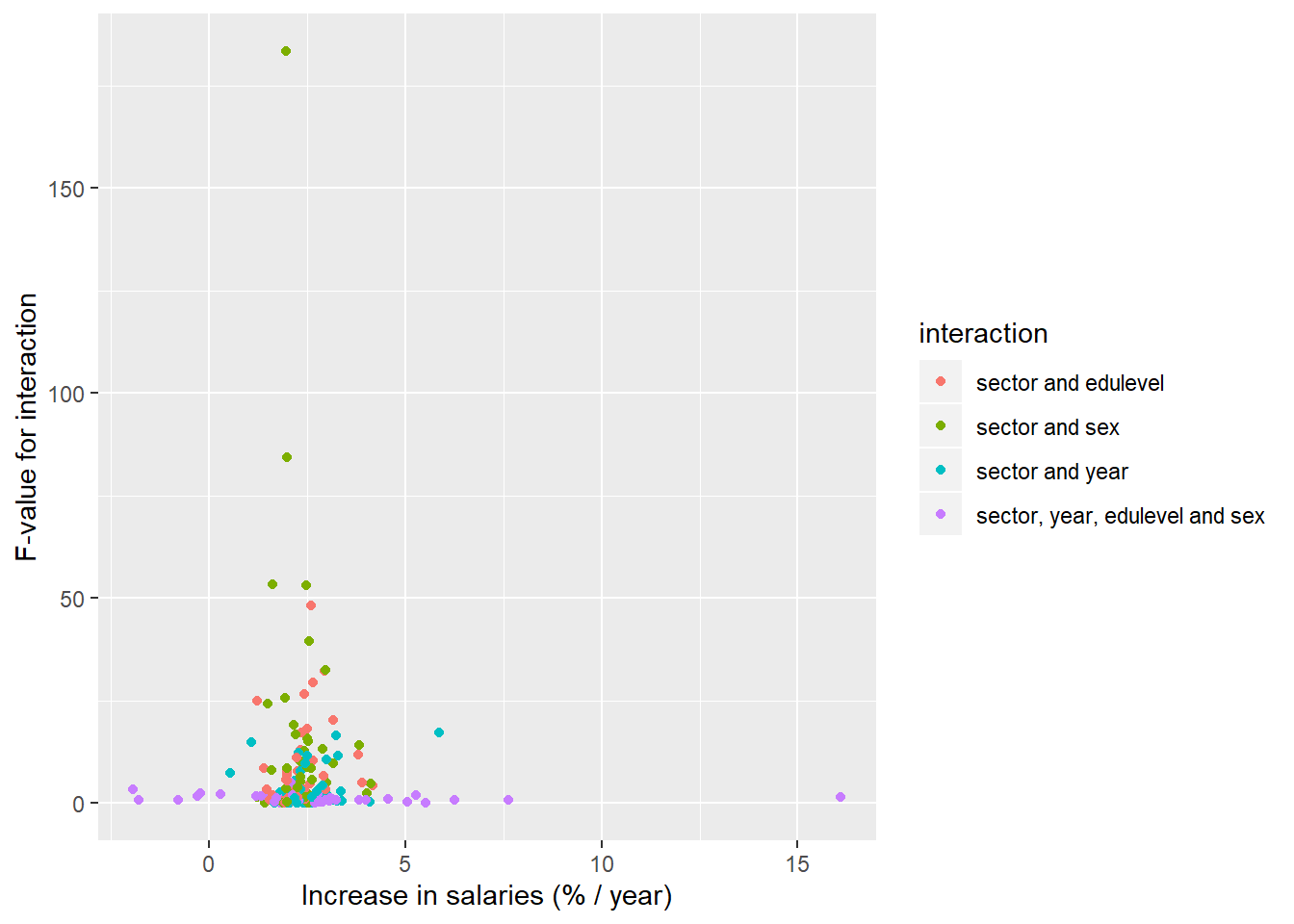
Figure 2: The significance of the interaction between sector, edulevel, year and sex on the salary in Sweden, a comparison between different occupational groups, Year 2014 - 2018
The tables with all occupational groups sorted by F-value in descending order.
merge(summary_table, anova_table, c("ssyk", "interaction"), all = TRUE) %>%
  filter (term.x == "year_n") %>%
  filter (term.y == "sector") %>%
  filter (interaction == "none") %>%
  mutate (estimate = (exp(estimate) - 1) * 100) %>%
  select (ssyk, estimate, statistic.y, interaction) %>%
  rename (`F-value` = statistic.y) %>%
  rename (`Increase in salary` = estimate) %>%
  arrange (desc (`F-value`)) %>%
  knitr::kable(
    booktabs = TRUE,
caption = 'Correlation for F-value (sector) and the yearly increase in salaries')| ssyk | Increase in salary | F-value | interaction |
|---|---|---|---|
| 242 Organisation analysts, policy administrators and human resource specialists | 1.609869 | 515.5748558 | none |
| 819 Process control technicians | 2.250895 | 467.4732796 | none |
| 251 ICT architects, systems analysts and test managers | 2.217446 | 465.2253589 | none |
| 331 Financial and accounting associate professionals | 1.964825 | 340.2901702 | none |
| 962 Newspaper distributors, janitors and other service workers | 1.971413 | 336.7676606 | none |
| 334 Administrative and specialized secretaries | 2.410127 | 333.7196510 | none |
| 351 ICT operations and user support technicians | 2.474549 | 305.6052807 | none |
| 241 Accountants, financial analysts and fund managers | 2.534461 | 251.4058600 | none |
| 335 Tax and related government associate professionals | 2.586686 | 250.8147705 | none |
| 515 Building caretakers and related workers | 2.522386 | 250.0742967 | none |
| 321 Medical and pharmaceutical technicians | 2.493038 | 230.0064060 | none |
| 213 Biologists, pharmacologists and specialists in agriculture and forestry | 2.303600 | 228.0668837 | none |
| 134 Architectural and engineering managers | 3.161068 | 226.5669850 | none |
| 333 Business services agents | 3.001597 | 222.9774594 | none |
| 411 Office assistants and other secretaries | 2.227235 | 214.6750980 | none |
| 243 Marketing and public relations professionals | 1.481519 | 179.3099186 | none |
| 264 Authors, journalists and linguists | 2.046538 | 164.8394018 | none |
| 129 Administration and service managers not elsewhere classified | 4.059900 | 158.7687951 | none |
| 342 Athletes, fitness instructors and recreational workers | 1.586943 | 132.1816646 | none |
| 159 Other social services managers | 2.541205 | 69.9268014 | none |
| 123 Administration and planning managers | 3.849200 | 50.0164438 | none |
| 541 Other surveillance and security workers | 2.460130 | 41.9287342 | none |
| 235 Teaching professionals not elsewhere classified | 1.415591 | 40.1919620 | none |
| 911 Cleaners and helpers | 1.938366 | 35.3850213 | none |
| 533 Health care assistants | 2.157379 | 22.0488822 | none |
| 534 Attendants, personal assistants and related workers | 1.959595 | 21.6985964 | none |
| 332 Insurance advisers, sales and purchasing agents | 2.637486 | 19.1041252 | none |
| 131 Information and communications technology service managers | 4.000609 | 17.0841502 | none |
| 311 Physical and engineering science technicians | 2.325958 | 16.5471030 | none |
| 214 Engineering professionals | 2.626260 | 15.6152029 | none |
| 432 Stores and transport clerks | 1.231854 | 13.9155189 | none |
| 723 Machinery mechanics and fitters | 2.362984 | 12.5847785 | none |
| 532 Personal care workers in health services | 2.906578 | 6.3336230 | none |
| 512 Cooks and cold-buffet managers | 2.483280 | 5.4612144 | none |
| 732 Printing trades workers | 2.158854 | 5.2405535 | none |
| 234 Primary- and pre-school teachers | 2.985653 | 4.6801860 | none |
| 422 Client information clerks | 2.527801 | 1.7881181 | none |
| 531 Child care workers and teachers aides | 1.881615 | 0.8334164 | none |
| 611 Market gardeners and crop growers | 1.980288 | 0.3732826 | none |
| 341 Social work and religious associate professionals | 2.357787 | 0.0276157 | none |
| 941 Fast-food workers, food preparation assistants | 1.981512 | 0.0046670 | none |
merge(summary_table, anova_table, c("ssyk", "interaction"), all = TRUE) %>%
  filter (term.x == "year_n") %>%
  filter (contcol.y > 0) %>%
  filter (interaction == "sector and sex") %>%
  mutate (estimate = (exp(estimate) - 1) * 100) %>%
  select (ssyk, estimate, statistic.y, interaction) %>%
  rename (`F-value` = statistic.y) %>%
  rename (`Increase in salary` = estimate) %>%
  arrange (desc (`F-value`)) %>%
  knitr::kable(
    booktabs = TRUE,
caption = 'Correlation for F-value (sector and sex) and the yearly increase in salaries')| ssyk | Increase in salary | F-value | interaction |
|---|---|---|---|
| 911 Cleaners and helpers | 1.966955 | 183.3539258 | sector and sex |
| 331 Financial and accounting associate professionals | 1.988628 | 84.3723061 | sector and sex |
| 342 Athletes, fitness instructors and recreational workers | 1.609407 | 53.2856268 | sector and sex |
| 351 ICT operations and user support technicians | 2.474549 | 53.1541368 | sector and sex |
| 241 Accountants, financial analysts and fund managers | 2.549161 | 39.5233707 | sector and sex |
| 333 Business services agents | 2.952973 | 32.5926396 | sector and sex |
| 611 Market gardeners and crop growers | 1.936338 | 25.7248443 | sector and sex |
| 243 Marketing and public relations professionals | 1.489860 | 24.3260135 | sector and sex |
| 533 Health care assistants | 2.157379 | 19.0714901 | sector and sex |
| 732 Printing trades workers | 2.207617 | 16.8065594 | sector and sex |
| 512 Cooks and cold-buffet managers | 2.497408 | 15.7408059 | sector and sex |
| 159 Other social services managers | 2.511558 | 15.1529257 | sector and sex |
| 123 Administration and planning managers | 3.819995 | 14.2436097 | sector and sex |
| 532 Personal care workers in health services | 2.899482 | 13.1974037 | sector and sex |
| 334 Administrative and specialized secretaries | 2.416957 | 12.8317750 | sector and sex |
| 213 Biologists, pharmacologists and specialists in agriculture and forestry | 2.317893 | 10.2339741 | sector and sex |
| 134 Architectural and engineering managers | 3.161068 | 9.7816667 | sector and sex |
| 321 Medical and pharmaceutical technicians | 2.493038 | 8.6670096 | sector and sex |
| 941 Fast-food workers, food preparation assistants | 1.989465 | 8.6486138 | sector and sex |
| 335 Tax and related government associate professionals | 2.586686 | 8.4427211 | sector and sex |
| 242 Organisation analysts, policy administrators and human resource specialists | 1.594999 | 8.1271264 | sector and sex |
| 723 Machinery mechanics and fitters | 2.337983 | 6.4299201 | sector and sex |
| 332 Insurance advisers, sales and purchasing agents | 2.627736 | 5.7400150 | sector and sex |
| 311 Physical and engineering science technicians | 2.316138 | 5.3473607 | sector and sex |
| 234 Primary- and pre-school teachers | 2.999161 | 5.0012138 | sector and sex |
| 129 Administration and service managers not elsewhere classified | 4.121066 | 4.6687219 | sector and sex |
| 819 Process control technicians | 2.250895 | 3.7631281 | sector and sex |
| 534 Attendants, personal assistants and related workers | 1.959595 | 3.5292601 | sector and sex |
| 131 Information and communications technology service managers | 4.029303 | 2.5233240 | sector and sex |
| 264 Authors, journalists and linguists | 2.033203 | 2.5032667 | sector and sex |
| 341 Social work and religious associate professionals | 2.357787 | 2.2988889 | sector and sex |
| 251 ICT architects, systems analysts and test managers | 2.217446 | 2.1823519 | sector and sex |
| 422 Client information clerks | 2.519631 | 2.1300830 | sector and sex |
| 432 Stores and transport clerks | 1.231854 | 1.5040767 | sector and sex |
| 541 Other surveillance and security workers | 2.457007 | 1.3945913 | sector and sex |
| 214 Engineering professionals | 2.629057 | 1.3225970 | sector and sex |
| 962 Newspaper distributors, janitors and other service workers | 1.971413 | 0.3480210 | sector and sex |
| 531 Child care workers and teachers aides | 1.879581 | 0.1432868 | sector and sex |
| 515 Building caretakers and related workers | 2.522844 | 0.1379141 | sector and sex |
| 235 Teaching professionals not elsewhere classified | 1.424488 | 0.0670314 | sector and sex |
| 411 Office assistants and other secretaries | 2.227235 | 0.0001653 | sector and sex |
merge(summary_table, anova_table, c("ssyk", "interaction"), all = TRUE) %>%
  filter (term.x == "year_n") %>%
  filter (contcol.y > 0) %>%
  filter (interaction == "sector and edulevel") %>%
  mutate (estimate = (exp(estimate) - 1) * 100) %>%
  select (ssyk, estimate, statistic.y, interaction) %>%
  rename (`F-value` = statistic.y) %>%
  rename (`Increase in salary` = estimate) %>%
  arrange (desc (`F-value`)) %>%
  knitr::kable(
    booktabs = TRUE,
caption = 'Correlation for F-value (sector and edulevel) and the yearly increase in salaries')| ssyk | Increase in salary | F-value | interaction |
|---|---|---|---|
| 335 Tax and related government associate professionals | 2.586686 | 48.2902588 | sector and edulevel |
| 234 Primary- and pre-school teachers | 2.936162 | 32.3560802 | sector and edulevel |
| 214 Engineering professionals | 2.636843 | 29.4462376 | sector and edulevel |
| 332 Insurance advisers, sales and purchasing agents | 2.420632 | 26.7105578 | sector and edulevel |
| 432 Stores and transport clerks | 1.231854 | 24.9194979 | sector and edulevel |
| 134 Architectural and engineering managers | 3.161068 | 20.3665858 | sector and edulevel |
| 321 Medical and pharmaceutical technicians | 2.493038 | 18.1556092 | sector and edulevel |
| 723 Machinery mechanics and fitters | 2.358171 | 17.3272819 | sector and edulevel |
| 311 Physical and engineering science technicians | 2.330300 | 12.9686992 | sector and edulevel |
| 123 Administration and planning managers | 3.809019 | 11.7436022 | sector and edulevel |
| 732 Printing trades workers | 2.220728 | 11.0453452 | sector and edulevel |
| 241 Accountants, financial analysts and fund managers | 2.647068 | 10.5100504 | sector and edulevel |
| 235 Teaching professionals not elsewhere classified | 1.396076 | 8.6264575 | sector and edulevel |
| 213 Biologists, pharmacologists and specialists in agriculture and forestry | 2.264110 | 7.7952190 | sector and edulevel |
| 941 Fast-food workers, food preparation assistants | 1.981512 | 7.5766373 | sector and edulevel |
| 331 Financial and accounting associate professionals | 1.980338 | 6.9758948 | sector and edulevel |
| 532 Personal care workers in health services | 2.919933 | 6.6231457 | sector and edulevel |
| 534 Attendants, personal assistants and related workers | 1.959595 | 5.7464596 | sector and edulevel |
| 962 Newspaper distributors, janitors and other service workers | 1.971413 | 5.4435379 | sector and edulevel |
| 131 Information and communications technology service managers | 3.908111 | 4.9661376 | sector and edulevel |
| 159 Other social services managers | 2.565523 | 4.7197836 | sector and edulevel |
| 129 Administration and service managers not elsewhere classified | 4.160995 | 4.3062655 | sector and edulevel |
| 251 ICT architects, systems analysts and test managers | 2.209131 | 3.5539841 | sector and edulevel |
| 512 Cooks and cold-buffet managers | 2.435903 | 3.4242806 | sector and edulevel |
| 333 Business services agents | 2.955970 | 3.3635706 | sector and edulevel |
| 243 Marketing and public relations professionals | 1.473064 | 3.2639790 | sector and edulevel |
| 264 Authors, journalists and linguists | 2.043677 | 3.0449469 | sector and edulevel |
| 334 Administrative and specialized secretaries | 2.387467 | 2.8528940 | sector and edulevel |
| 422 Client information clerks | 2.527801 | 2.3007696 | sector and edulevel |
| 242 Organisation analysts, policy administrators and human resource specialists | 1.612900 | 1.9599904 | sector and edulevel |
| 351 ICT operations and user support technicians | 2.474549 | 1.5903279 | sector and edulevel |
| 819 Process control technicians | 2.250895 | 1.5586112 | sector and edulevel |
| 341 Social work and religious associate professionals | 2.357787 | 1.3263497 | sector and edulevel |
| 611 Market gardeners and crop growers | 2.016345 | 1.2719035 | sector and edulevel |
| 541 Other surveillance and security workers | 2.460130 | 1.0672924 | sector and edulevel |
| 411 Office assistants and other secretaries | 2.227235 | 1.0114046 | sector and edulevel |
| 515 Building caretakers and related workers | 2.526100 | 0.8254389 | sector and edulevel |
| 342 Athletes, fitness instructors and recreational workers | 1.540952 | 0.8230839 | sector and edulevel |
| 531 Child care workers and teachers aides | 1.897863 | 0.7969406 | sector and edulevel |
| 533 Health care assistants | 2.157379 | 0.5425248 | sector and edulevel |
| 911 Cleaners and helpers | 1.938366 | 0.0965584 | sector and edulevel |
merge(summary_table, anova_table, c("ssyk", "interaction"), all = TRUE) %>%
  filter (term.x == "year_n") %>%
  filter (contcol.y > 0) %>%
  filter (interaction == "sector and year") %>%
  mutate (estimate = (exp(estimate) - 1) * 100) %>%
  select (ssyk, estimate, statistic.y, interaction) %>%
  rename (`F-value` = statistic.y) %>%
  rename (`Increase in salary` = estimate) %>%
  arrange (desc (`F-value`)) %>%
  knitr::kable(
    booktabs = TRUE,
caption = 'Correlation for F-value (sector and year) and the yearly increase in salaries')| ssyk | Increase in salary | F-value | interaction |
|---|---|---|---|
| 129 Administration and service managers not elsewhere classified | 5.8528187 | 17.1667457 | sector and year |
| 351 ICT operations and user support technicians | 3.2455362 | 16.6101284 | sector and year |
| 334 Administrative and specialized secretaries | 1.0672775 | 14.9508269 | sector and year |
| 534 Attendants, personal assistants and related workers | 2.2769477 | 12.4036331 | sector and year |
| 422 Client information clerks | 3.2733483 | 11.6812523 | sector and year |
| 962 Newspaper distributors, janitors and other service workers | 2.4907346 | 11.5673142 | sector and year |
| 264 Authors, journalists and linguists | 2.9905121 | 10.5945994 | sector and year |
| 531 Child care workers and teachers aides | 2.4510286 | 9.5936100 | sector and year |
| 242 Organisation analysts, policy administrators and human resource specialists | 2.3355826 | 7.7816291 | sector and year |
| 432 Stores and transport clerks | 0.5332567 | 7.4196762 | sector and year |
| 243 Marketing and public relations professionals | 2.1828057 | 5.5660180 | sector and year |
| 732 Printing trades workers | 2.8825380 | 4.3716553 | sector and year |
| 213 Biologists, pharmacologists and specialists in agriculture and forestry | 2.8099783 | 3.6786224 | sector and year |
| 611 Market gardeners and crop growers | 2.3161238 | 3.3017939 | sector and year |
| 131 Information and communications technology service managers | 3.3504930 | 2.8750373 | sector and year |
| 532 Personal care workers in health services | 2.7411030 | 2.8290655 | sector and year |
| 235 Teaching professionals not elsewhere classified | 1.8047571 | 2.7841902 | sector and year |
| 311 Physical and engineering science technicians | 2.8608741 | 2.6173373 | sector and year |
| 533 Health care assistants | 1.9920113 | 2.2486864 | sector and year |
| 214 Engineering professionals | 3.0209963 | 2.0446973 | sector and year |
| 723 Machinery mechanics and fitters | 2.6258864 | 1.4272778 | sector and year |
| 515 Building caretakers and related workers | 2.3423357 | 1.3492650 | sector and year |
| 321 Medical and pharmaceutical technicians | 2.1376334 | 1.2494762 | sector and year |
| 941 Fast-food workers, food preparation assistants | 2.1906312 | 1.1458297 | sector and year |
| 234 Primary- and pre-school teachers | 3.1522849 | 0.8075167 | sector and year |
| 411 Office assistants and other secretaries | 2.4217447 | 0.7799156 | sector and year |
| 241 Accountants, financial analysts and fund managers | 2.2625663 | 0.7751592 | sector and year |
| 541 Other surveillance and security workers | 2.3018747 | 0.6646888 | sector and year |
| 134 Architectural and engineering managers | 3.3811821 | 0.5852232 | sector and year |
| 333 Business services agents | 3.2520012 | 0.5424390 | sector and year |
| 335 Tax and related government associate professionals | 2.3986233 | 0.3139375 | sector and year |
| 123 Administration and planning managers | 4.0945884 | 0.2682143 | sector and year |
| 911 Cleaners and helpers | 2.0082873 | 0.2021948 | sector and year |
| 341 Social work and religious associate professionals | 2.3994292 | 0.0754320 | sector and year |
| 342 Athletes, fitness instructors and recreational workers | 1.6673896 | 0.0633281 | sector and year |
| 512 Cooks and cold-buffet managers | 2.4249631 | 0.0494622 | sector and year |
| 819 Process control technicians | 2.2225873 | 0.0378303 | sector and year |
| 331 Financial and accounting associate professionals | 2.0557505 | 0.0377336 | sector and year |
| 251 ICT architects, systems analysts and test managers | 2.2536138 | 0.0294035 | sector and year |
| 332 Insurance advisers, sales and purchasing agents | 2.6015664 | 0.0125275 | sector and year |
| 159 Other social services managers | 2.5487758 | 0.0013436 | sector and year |
merge(summary_table, anova_table, c("ssyk", "interaction"), all = TRUE) %>%
  filter (term.x == "year_n") %>%
  filter (contcol.y > 1) %>%
  filter (interaction == "sector, year, edulevel and sex") %>%
  filter (!(contcol.y < 3 & interaction == "sector, year, edulevel and sex")) %>%
  mutate (estimate = (exp(estimate) - 1) * 100) %>%
  select (ssyk, estimate, statistic.y, interaction) %>%
  rename (`F-value` = statistic.y) %>%
  rename (`Increase in salary` = estimate) %>%
  arrange (desc (`F-value`)) %>%
  knitr::kable(
    booktabs = TRUE,
caption = 'Correlation for F-value (sector, year, edulevel and sex) and the yearly increase in salaries')| ssyk | Increase in salary | F-value | interaction |
|---|---|---|---|
| 264 Authors, journalists and linguists | 2.0717871 | 5.0646298 | sector, year, edulevel and sex |
| 311 Physical and engineering science technicians | -1.9358596 | 3.3593399 | sector, year, edulevel and sex |
| 159 Other social services managers | 2.1339049 | 2.5206357 | sector, year, edulevel and sex |
| 134 Architectural and engineering managers | -0.2221716 | 2.4150753 | sector, year, edulevel and sex |
| 331 Financial and accounting associate professionals | 0.2989757 | 2.2892768 | sector, year, edulevel and sex |
| 342 Athletes, fitness instructors and recreational workers | 2.7799167 | 2.1976399 | sector, year, edulevel and sex |
| 214 Engineering professionals | 5.2732904 | 1.9988132 | sector, year, edulevel and sex |
| 723 Machinery mechanics and fitters | 2.1334983 | 1.8843643 | sector, year, edulevel and sex |
| 432 Stores and transport clerks | -0.2883737 | 1.8215339 | sector, year, edulevel and sex |
| 241 Accountants, financial analysts and fund managers | 2.6268377 | 1.8184489 | sector, year, edulevel and sex |
| 533 Health care assistants | 1.3176280 | 1.6357939 | sector, year, edulevel and sex |
| 911 Cleaners and helpers | 1.1875630 | 1.6319874 | sector, year, edulevel and sex |
| 129 Administration and service managers not elsewhere classified | 16.0932403 | 1.5716145 | sector, year, edulevel and sex |
| 512 Cooks and cold-buffet managers | 2.2335677 | 1.4882138 | sector, year, edulevel and sex |
| 242 Organisation analysts, policy administrators and human resource specialists | 1.9377802 | 1.4494844 | sector, year, edulevel and sex |
| 234 Primary- and pre-school teachers | 2.6286211 | 1.4408203 | sector, year, edulevel and sex |
| 235 Teaching professionals not elsewhere classified | 1.4806649 | 1.4162230 | sector, year, edulevel and sex |
| 532 Personal care workers in health services | 3.0809717 | 1.3439893 | sector, year, edulevel and sex |
| 962 Newspaper distributors, janitors and other service workers | 1.7217534 | 1.3344044 | sector, year, edulevel and sex |
| 332 Insurance advisers, sales and purchasing agents | 4.5515134 | 0.9604905 | sector, year, edulevel and sex |
| 123 Administration and planning managers | 1.6860436 | 0.9155189 | sector, year, edulevel and sex |
| 541 Other surveillance and security workers | 3.1372549 | 0.9113280 | sector, year, edulevel and sex |
| 213 Biologists, pharmacologists and specialists in agriculture and forestry | 2.0956711 | 0.9044780 | sector, year, edulevel and sex |
| 422 Client information clerks | 7.6231100 | 0.8611877 | sector, year, edulevel and sex |
| 515 Building caretakers and related workers | 3.8284291 | 0.8343329 | sector, year, edulevel and sex |
| 334 Administrative and specialized secretaries | -1.8021942 | 0.7940149 | sector, year, edulevel and sex |
| 531 Child care workers and teachers aides | 2.9556278 | 0.7580341 | sector, year, edulevel and sex |
| 131 Information and communications technology service managers | 6.2536436 | 0.7429188 | sector, year, edulevel and sex |
| 243 Marketing and public relations professionals | -0.7939038 | 0.7338409 | sector, year, edulevel and sex |
| 351 ICT operations and user support technicians | 3.2312302 | 0.7188959 | sector, year, edulevel and sex |
| 732 Printing trades workers | 3.9993823 | 0.6905319 | sector, year, edulevel and sex |
| 321 Medical and pharmaceutical technicians | 2.2164674 | 0.6326293 | sector, year, edulevel and sex |
| 611 Market gardeners and crop growers | 2.2753348 | 0.6157880 | sector, year, edulevel and sex |
| 341 Social work and religious associate professionals | 3.0666620 | 0.5266982 | sector, year, edulevel and sex |
| 941 Fast-food workers, food preparation assistants | 2.7940568 | 0.4253642 | sector, year, edulevel and sex |
| 335 Tax and related government associate professionals | 5.0470456 | 0.3217115 | sector, year, edulevel and sex |
| 251 ICT architects, systems analysts and test managers | 2.9031256 | 0.2684425 | sector, year, edulevel and sex |
| 819 Process control technicians | 1.6741717 | 0.2603997 | sector, year, edulevel and sex |
| 333 Business services agents | 1.8143344 | 0.1540308 | sector, year, edulevel and sex |
| 411 Office assistants and other secretaries | 5.5231019 | 0.0911334 | sector, year, edulevel and sex |
| 534 Attendants, personal assistants and related workers | 2.6927719 | 0.0899580 | sector, year, edulevel and sex |
Let’s check what we have found.
temp <- tbnum %>%
  filter(`occuptional  (SSYK 2012)` == "242 Organisation analysts, policy administrators and human resource specialists")

model <- lm (log(salary) ~ year_n + eduyears + sector + sex, data = temp)

plot_model(model, type = "pred", terms = c("eduyears", "sector"))
## Model has log-transformed response. Back-transforming predictions to original response scale. Standard errors are still on the log-scale.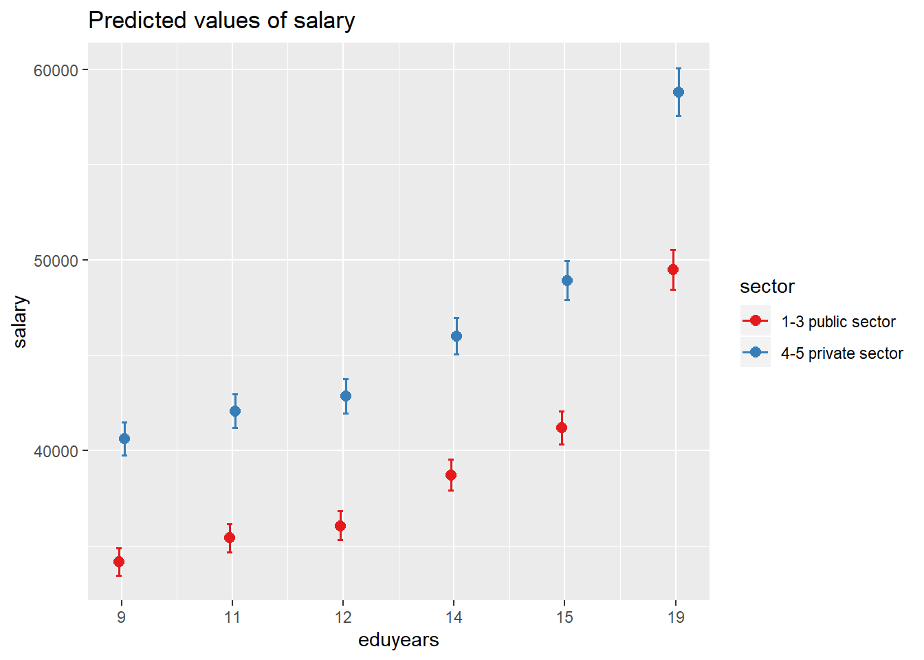
Figure 3: Highest F-value sector, Organisation analysts, policy administrators and human resource specialists
temp <- tbnum %>%
  filter(`occuptional  (SSYK 2012)` == "941 Fast-food workers, food preparation assistants")

model <-lm (log(salary) ~ year_n + eduyears + sector + sex, data = temp)

plot_model(model, type = "pred", terms = c("eduyears", "sector"))
## Model has log-transformed response. Back-transforming predictions to original response scale. Standard errors are still on the log-scale.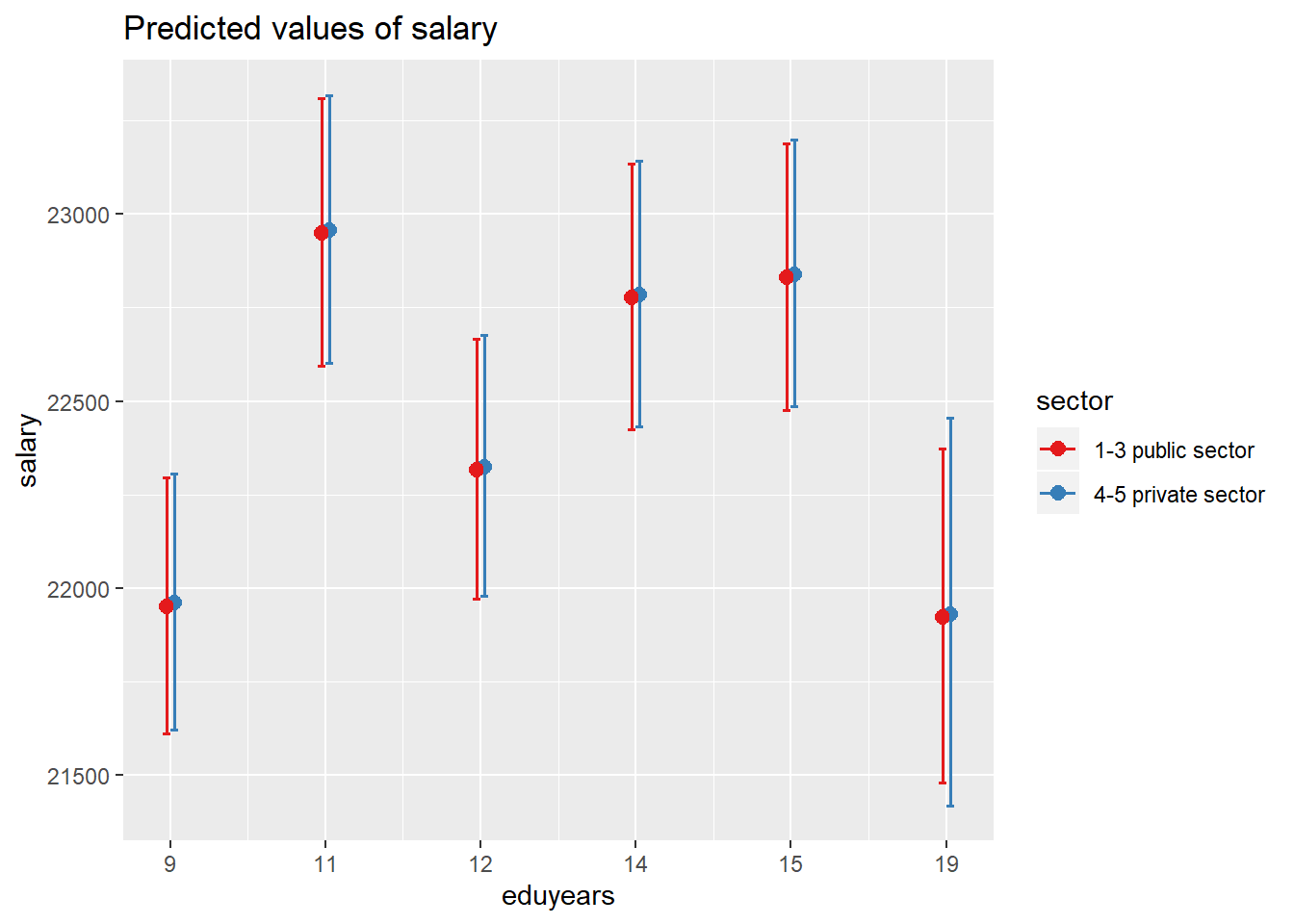
Figure 4: Lowest F-value sector, Fast-food workers, food preparation assistants
temp <- tbnum %>%
  filter(`occuptional  (SSYK 2012)` == "911 Cleaners and helpers")

model <- lm (log(salary) ~ year_n + eduyears + sector * sex, data = temp)

plot_model(model, type = "pred", terms = c("eduyears", "sex", "sector"))
## Model has log-transformed response. Back-transforming predictions to original response scale. Standard errors are still on the log-scale.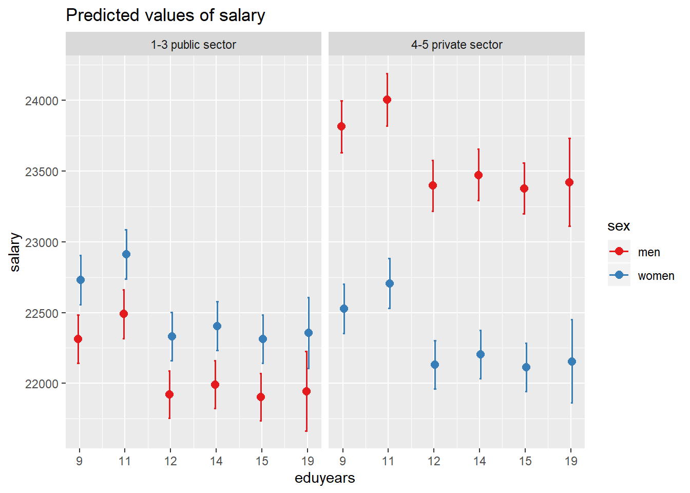
Figure 5: Highest F-value interaction sector and gender, Cleaners and helpers
temp <- tbnum %>%
  filter(`occuptional  (SSYK 2012)` == "411 Office assistants and other secretaries")

model <- lm (log(salary) ~ year_n + eduyears + sector * sex, data = temp)

plot_model(model, type = "pred", terms = c("eduyears", "sex", "sector"))
## Model has log-transformed response. Back-transforming predictions to original response scale. Standard errors are still on the log-scale.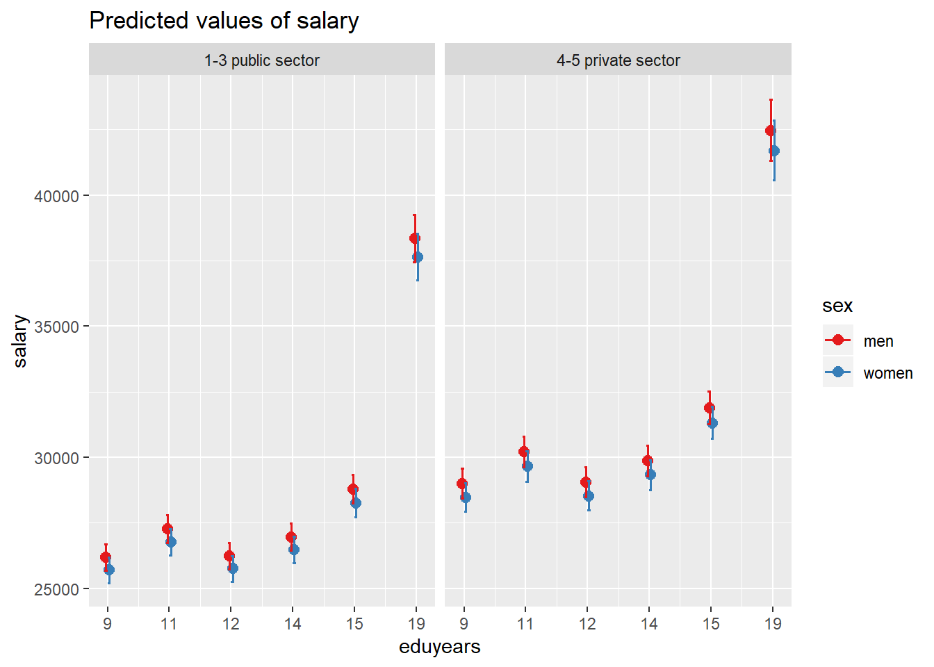
Figure 6: Lowest F-value interaction sector and gender, Office assistants and other secretaries
temp <- tbnum %>%
  filter(`occuptional  (SSYK 2012)` == "335 Tax and related government associate professionals")

model <- lm (log(salary) ~ year_n + eduyears * sector + sex, data = temp)

plot_model(model, type = "pred", terms = c("eduyears", "sector"))
## Warning in predict.lm(model, newdata = fitfram, type = "response", se.fit =
## se, : prediction from a rank-deficient fit may be misleading## Model has log-transformed response. Back-transforming predictions to original response scale. Standard errors are still on the log-scale.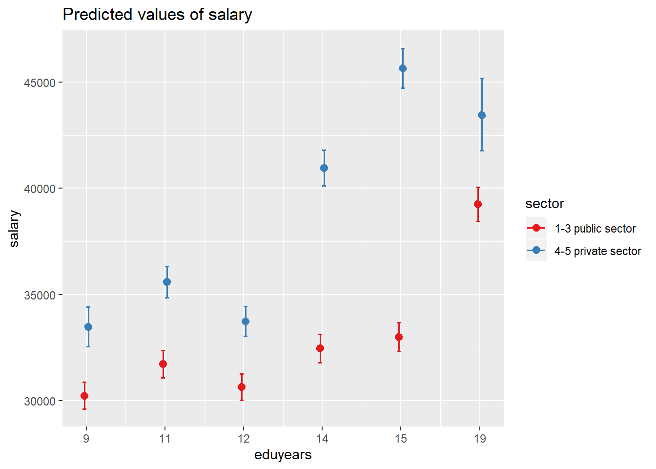
Figure 7: Highest F-value interaction sector and edulevel, Tax and related government associate professionals
temp <- tbnum %>%
  filter(`occuptional  (SSYK 2012)` == "911 Cleaners and helpers")

model <- lm (log(salary) ~ year_n + eduyears * sector + sex, data = temp)

plot_model(model, type = "pred", terms = c("eduyears", "sector"))
## Warning in predict.lm(model, newdata = fitfram, type = "response", se.fit =
## se, : prediction from a rank-deficient fit may be misleading## Model has log-transformed response. Back-transforming predictions to original response scale. Standard errors are still on the log-scale.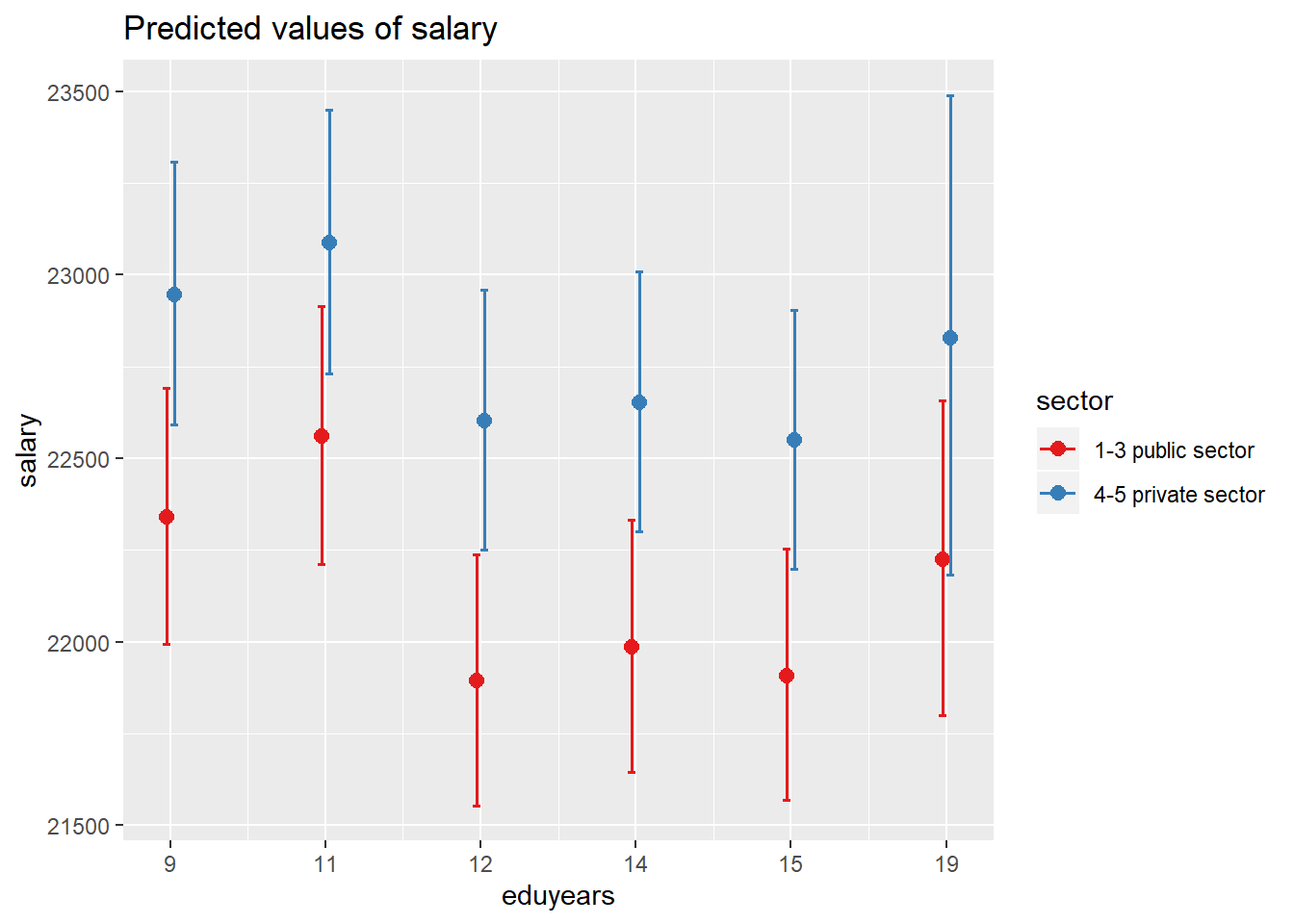
Figure 8: Lowest F-value interaction sector and edulevel, Cleaners and helpers
temp <- tbnum %>%
  filter(`occuptional  (SSYK 2012)` == "129 Administration and service managers not elsewhere classified")

model <- lm (log(salary) ~ year_n * sector + eduyears + sex, data = temp)

plot_model(model, type = "pred", terms = c("eduyears", "year_n", "sector"))
## Model has log-transformed response. Back-transforming predictions to original response scale. Standard errors are still on the log-scale.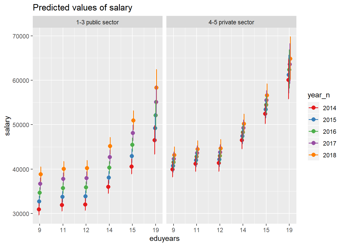
Figure 9: Highest F-value interaction sector and year, Administration and service managers not elsewhere classified
temp <- tbnum %>%
  filter(`occuptional  (SSYK 2012)` == "159 Other social services managers")

model <- lm (log(salary) ~ year_n * sector + eduyears + sex, data = temp)

plot_model(model, type = "pred", terms = c("eduyears", "year_n", "sector"))
## Model has log-transformed response. Back-transforming predictions to original response scale. Standard errors are still on the log-scale.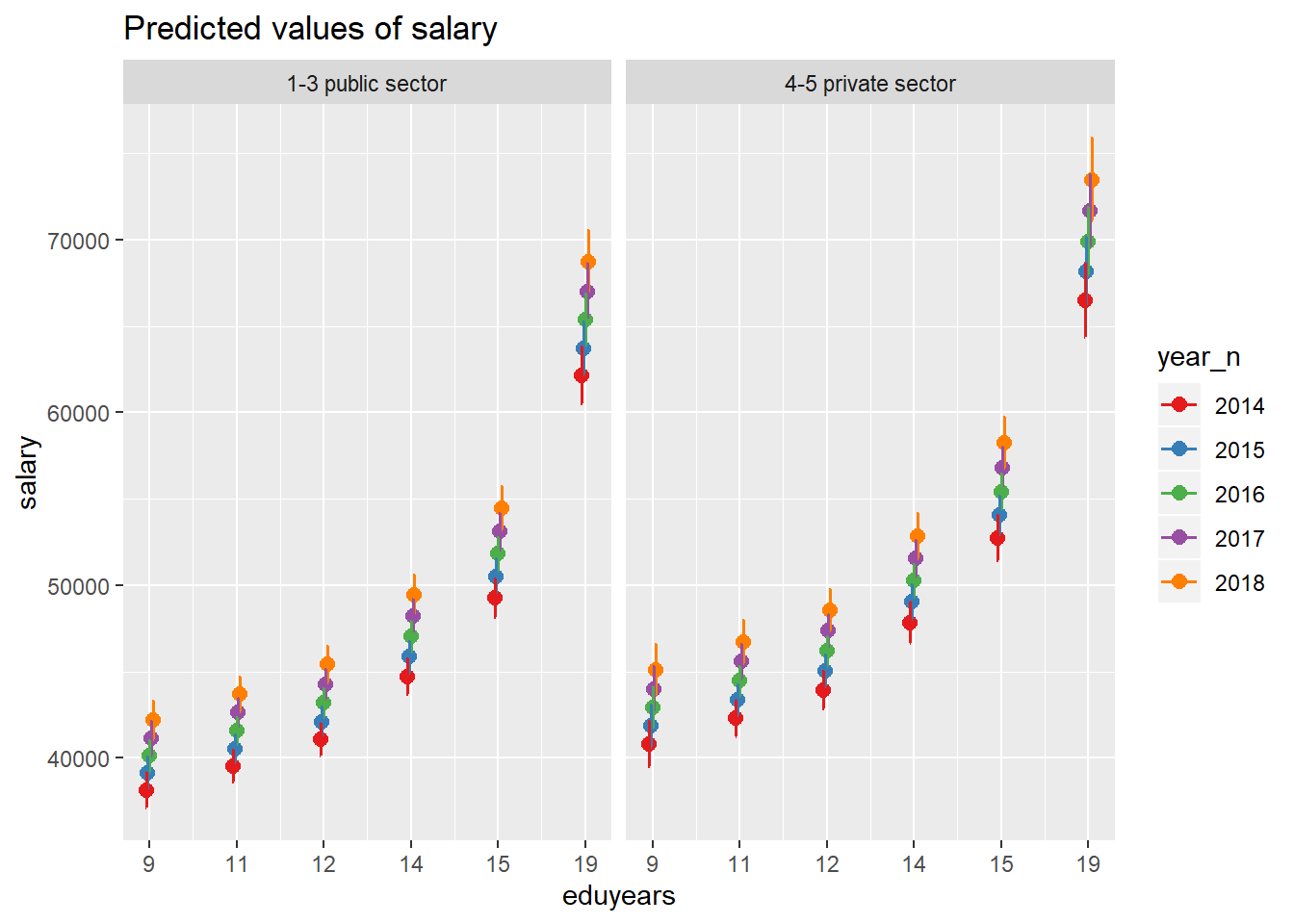
Figure 10: Lowest F-value interaction sector and year, Other social services managers
temp <- tbnum %>%
  filter(`occuptional  (SSYK 2012)` == "264 Authors, journalists and linguists")

model <- lm (log(salary) ~ year_n * eduyears * sector * sex, data = temp)

plot_model(model, type = "pred", terms = c("eduyears", "year_n", "sex", "sector"))
## Warning in predict.lm(model, newdata = fitfram, type = "response", se.fit =
## se, : prediction from a rank-deficient fit may be misleading## Model has log-transformed response. Back-transforming predictions to original response scale. Standard errors are still on the log-scale.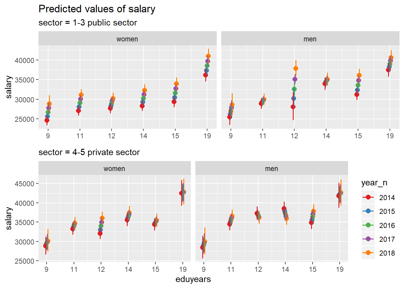
Figure 11: Highest F-value interaction sector, edulevel, year and gender, Authors, journalists and linguists
## TableGrob (2 x 1) "arrange": 2 grobs
##   z     cells    name           grob
## 1 1 (1-1,1-1) arrange gtable[layout]
## 2 2 (2-2,1-1) arrange gtable[layout]
temp <- tbnum %>%
filter(`occuptional (SSYK 2012)` == "534 Attendants, personal assistants and related workers")
model <- lm (log(salary) ~ year_n * eduyears * sector * sex, data = temp)
plot_model(model, type = "pred", terms = c("eduyears", "year_n", "sex", "sector"))## Warning in predict.lm(model, newdata = fitfram, type = "response", se.fit =
## se, : prediction from a rank-deficient fit may be misleading## Model has log-transformed response. Back-transforming predictions to original response scale. Standard errors are still on the log-scale.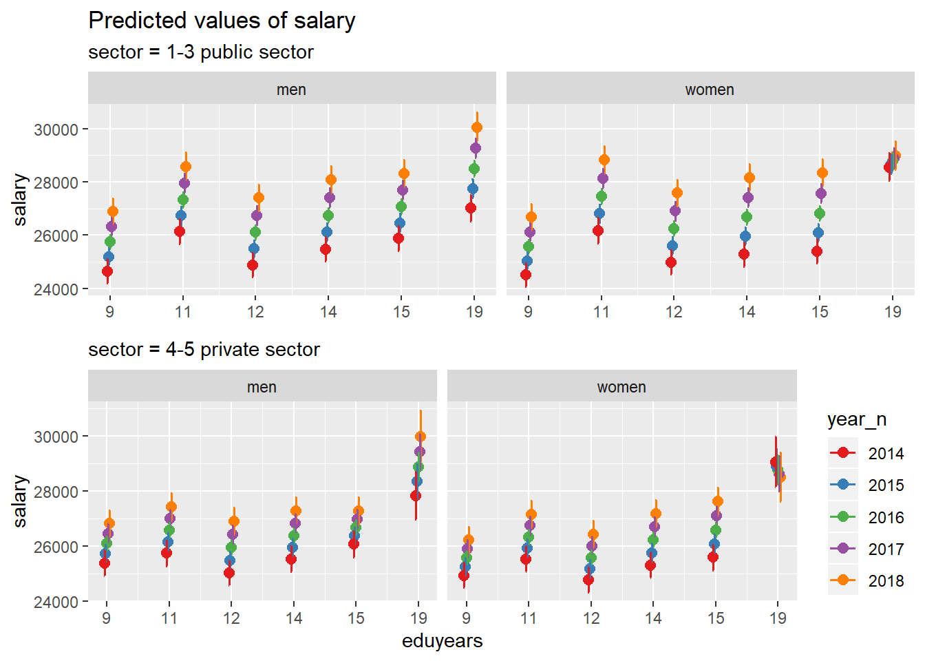
Figure 12: Lowest F-value interaction sector, edulevel, year and gender, Attendants, personal assistants and related workers
## TableGrob (2 x 1) "arrange": 2 grobs
##   z     cells    name           grob
## 1 1 (1-1,1-1) arrange gtable[layout]
## 2 2 (2-2,1-1) arrange gtable[layout]