The significance of population size, year, and per cent women on the education level in Sweden

In twelve posts I have analysed how different factors are related to salaries in Sweden with data from Statistics Sweden. In this post, I will analyse a new dataset from Statistics Sweden, population by region, age, level of education, sex and year. Not knowing exactly what to find I will use a criterion-based procedure to find the model that minimises the AIC. Then I will perform some test to see how robust the model is. Finally, I will plot the findings.

First, define libraries and functions.

library (tidyverse)

## -- Attaching packages -------------------------------------------------- tidyverse 1.3.0 --

## v ggplot2 3.2.1     v purrr   0.3.3
## v tibble  2.1.3     v dplyr   0.8.3
## v tidyr   1.0.2     v stringr 1.4.0
## v readr   1.3.1     v forcats 0.4.0

## -- Conflicts ----------------------------------------------------- tidyverse_conflicts() --
## x dplyr::filter() masks stats::filter()
## x dplyr::lag()    masks stats::lag()

library (broom)
library (car)

## Loading required package: carData

## 
## Attaching package: 'car'

## The following object is masked from 'package:dplyr':
## 
##     recode

## The following object is masked from 'package:purrr':
## 
##     some

library (sjPlot)

## Registered S3 methods overwritten by 'lme4':
##   method                          from
##   cooks.distance.influence.merMod car 
##   influence.merMod                car 
##   dfbeta.influence.merMod         car 
##   dfbetas.influence.merMod        car

library (leaps)
library (splines)
library (MASS)

## 
## Attaching package: 'MASS'

## The following object is masked from 'package:dplyr':
## 
##     select

library (mgcv)

## Loading required package: nlme

## 
## Attaching package: 'nlme'

## The following object is masked from 'package:dplyr':
## 
##     collapse

## This is mgcv 1.8-31. For overview type 'help("mgcv-package")'.

library (lmtest)

## Loading required package: zoo

## 
## Attaching package: 'zoo'

## The following objects are masked from 'package:base':
## 
##     as.Date, as.Date.numeric

library (earth)

## Warning: package 'earth' was built under R version 3.6.3

## Loading required package: Formula

## Loading required package: plotmo

## Warning: package 'plotmo' was built under R version 3.6.3

## Loading required package: plotrix

## Loading required package: TeachingDemos

## Warning: package 'TeachingDemos' was built under R version 3.6.3

library (acepack)

## Warning: package 'acepack' was built under R version 3.6.3

library (lspline)

## Warning: package 'lspline' was built under R version 3.6.3

library (lme4)

## Loading required package: Matrix

## 
## Attaching package: 'Matrix'

## The following objects are masked from 'package:tidyr':
## 
##     expand, pack, unpack

## 
## Attaching package: 'lme4'

## The following object is masked from 'package:nlme':
## 
##     lmList

library (pROC)

## Warning: package 'pROC' was built under R version 3.6.3

## Type 'citation("pROC")' for a citation.

## 
## Attaching package: 'pROC'

## The following objects are masked from 'package:stats':
## 
##     cov, smooth, var

readfile <- function (file1){read_csv (file1, col_types = cols(), locale = readr::locale (encoding = "latin1"), na = c("..", "NA")) %>%
  gather (starts_with("19"), starts_with("20"), key = "year", value = groupsize) %>%
  drop_na() %>%
  mutate (year_n = parse_number (year))
}

perc_women <- function(x){  
  ifelse (length(x) == 2, x[2] / (x[1] + x[2]), NA)
} 

nuts <- read.csv("nuts.csv") %>%
  mutate(NUTS2_sh = substr(NUTS2, 3, 4))

The data table is downloaded from Statistics Sweden. It is saved as a comma-delimited file without heading, UF0506A1.csv, http://www.statistikdatabasen.scb.se/pxweb/en/ssd/.

I will calculate the percentage of women in for the different education levels in the different regions for each year. In my later analysis I will use the number of people in each education level, region and year.

The table: Population 16-74 years of age by region, highest level of education, age and sex. Year 1985 - 2018 NUTS 2 level 2008- 10 year intervals (16-74)

tb <- readfile("UF0506A1.csv") %>%  
  mutate(edulevel = `level of education`) %>%
  group_by(edulevel, region, year, sex) %>%
  mutate(groupsize_all_ages = sum(groupsize)) %>%  
  group_by(edulevel, region, year) %>% 
  mutate (sum_edu_region_year = sum(groupsize)) %>%  
  mutate (perc_women = perc_women (groupsize_all_ages[1:2])) %>% 
  group_by(region, year) %>%
  mutate (sum_pop = sum(groupsize)) %>% rowwise() %>%
  mutate(age_l = unlist(lapply(strsplit(substr(age, 1, 5), "-"), strtoi))[1]) %>%
  rowwise() %>% 
  mutate(age_h = unlist(lapply(strsplit(substr(age, 1, 5), "-"), strtoi))[2]) %>%
  mutate(age_n = (age_l + age_h) / 2) %>%
  left_join(nuts %>% distinct (NUTS2_en, NUTS2_sh), by = c("region" = "NUTS2_en"))

## Warning: Column `region`/`NUTS2_en` joining character vector and factor,
## coercing into character vector

numedulevel <- read.csv("edulevel_1.csv") 

numedulevel %>%
  knitr::kable(
  booktabs = TRUE,
  caption = 'Initial approach, length of education')

Table 1: Initial approach, length of education
level.of.education	eduyears
primary and secondary education less than 9 years (ISCED97 1)	8
primary and secondary education 9-10 years (ISCED97 2)	9
upper secondary education, 2 years or less (ISCED97 3C)	11
upper secondary education 3 years (ISCED97 3A)	12
post-secondary education, less than 3 years (ISCED97 4+5B)	14
post-secondary education 3 years or more (ISCED97 5A)	15
post-graduate education (ISCED97 6)	19
no information about level of educational attainment	NA

tbnum <- tb %>% 
  right_join(numedulevel, by = c("level of education" = "level.of.education")) %>%
  filter(!is.na(eduyears)) %>% 
  drop_na()

## Warning: Column `level of education`/`level.of.education` joining character
## vector and factor, coercing into character vector

tbnum %>%
  ggplot () +  
    geom_point (mapping = aes(x = NUTS2_sh,y = perc_women, colour = year_n)) +
  facet_grid(. ~ eduyears)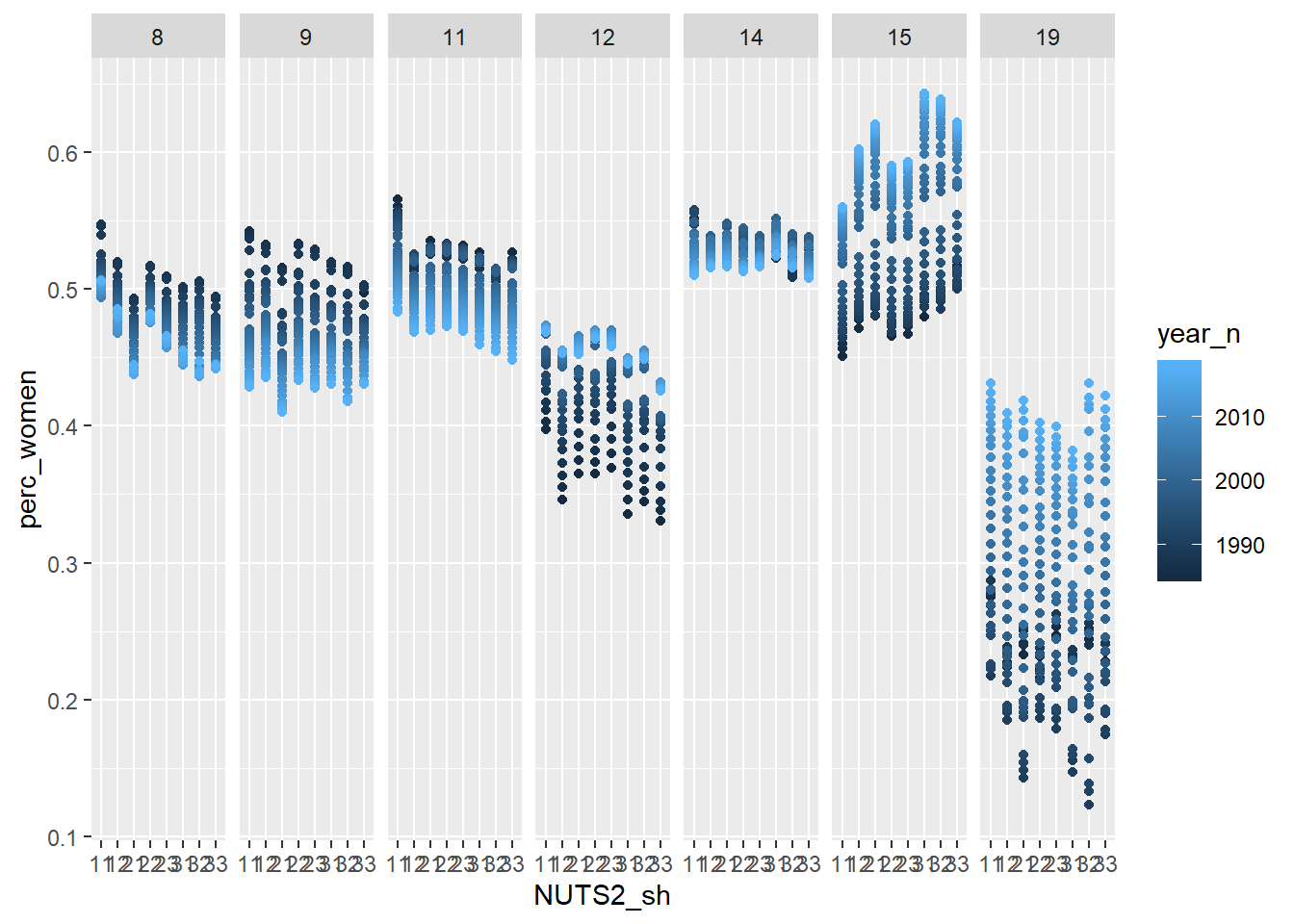

Figure 1: Population by region, level of education, percent women and year, Year 1985 - 2018

summary(tbnum)

##     region              age            level of education     sex           
##  Length:22848       Length:22848       Length:22848       Length:22848      
##  Class :character   Class :character   Class :character   Class :character  
##  Mode  :character   Mode  :character   Mode  :character   Mode  :character  
##                                                                             
##                                                                             
##                                                                             
##      year             groupsize         year_n       edulevel        
##  Length:22848       Min.   :    0   Min.   :1985   Length:22848      
##  Class :character   1st Qu.: 1634   1st Qu.:1993   Class :character  
##  Mode  :character   Median : 5646   Median :2002   Mode  :character  
##                     Mean   : 9559   Mean   :2002                     
##                     3rd Qu.:14027   3rd Qu.:2010                     
##                     Max.   :77163   Max.   :2018                     
##  groupsize_all_ages sum_edu_region_year   perc_women        sum_pop       
##  Min.   :    45     Min.   :   366      Min.   :0.1230   Min.   : 266057  
##  1st Qu.: 20033     1st Qu.: 40482      1st Qu.:0.4416   1st Qu.: 515306  
##  Median : 45592     Median : 90871      Median :0.4816   Median : 740931  
##  Mean   : 57353     Mean   :114706      Mean   :0.4641   Mean   : 823034  
##  3rd Qu.: 86203     3rd Qu.:172120      3rd Qu.:0.5217   3rd Qu.:1195658  
##  Max.   :271889     Max.   :486270      Max.   :0.6423   Max.   :1716160  
##      age_l           age_h        age_n         NUTS2_sh        
##  Min.   :16.00   Min.   :24   Min.   :20.00   Length:22848      
##  1st Qu.:25.00   1st Qu.:34   1st Qu.:29.50   Class :character  
##  Median :40.00   Median :49   Median :44.50   Mode  :character  
##  Mean   :40.17   Mean   :49   Mean   :44.58                     
##  3rd Qu.:55.00   3rd Qu.:64   3rd Qu.:59.50                     
##  Max.   :65.00   Max.   :74   Max.   :69.50                     
##     eduyears    
##  Min.   : 8.00  
##  1st Qu.: 9.00  
##  Median :12.00  
##  Mean   :12.57  
##  3rd Qu.:15.00  
##  Max.   :19.00

In a previous post, I approximated the number of years of education for every education level. Since this approximation is significant for the rest of the analysis I will see if I can do a better approximation. I use Multivariate Adaptive Regression Splines (MARS) to find the permutation of years of education, within the given limitations, which gives the highest adjusted R-Squared value. I choose not to calculate more combinations than between the age of 7 and 19 because I assessed it would take to much time. From the table, we can see that the R-Squared only gains from a higher education year for post-graduate education. A manual test shows that setting years of education to 22 gives a higher R-Squared without getting high residuals.

educomb <- as_tibble(t(combn(7:19,7))) %>% 
  filter((V6 - V4) > 2) %>% filter((V4 - V2) > 2) %>% 
  filter(V2 > 8) %>% 
  mutate(na = NA)

## Warning: `as_tibble.matrix()` requires a matrix with column names or a `.name_repair` argument. Using compatibility `.name_repair`.
## This warning is displayed once per session.

summary_table = vector()

for (i in 1:dim(educomb)[1]) {
  numedulevel[, 2] <- t(educomb[i,])

  suppressWarnings (tbnum <- tb %>% 
    right_join(numedulevel, by = c("level of education" = "level.of.education")) %>%
    filter(!is.na(eduyears)) %>% 
    drop_na())

  tbtest <- tbnum %>% 
    dplyr::select(eduyears, sum_pop, sum_edu_region_year, year_n, perc_women)

  mmod <- earth(eduyears ~ ., data = tbtest, nk = 12, degree = 2)

  summary_table <- rbind(summary_table, summary(mmod)$rsq)
}

which.max(summary_table)

## [1] 235

educomb[which.max(summary_table),] #235

## # A tibble: 1 x 8
##      V1    V2    V3    V4    V5    V6    V7 na   
##   <int> <int> <int> <int> <int> <int> <int> <lgl>
## 1     8     9    10    12    13    15    19 NA

numedulevel[, 2] <- t(educomb[235,])

numedulevel[7, 2] <- 22

numedulevel %>%
  knitr::kable(
  booktabs = TRUE,
  caption = 'Recalculated length of education')

Table 2: Recalculated length of education
level.of.education	eduyears
primary and secondary education less than 9 years (ISCED97 1)	8
primary and secondary education 9-10 years (ISCED97 2)	9
upper secondary education, 2 years or less (ISCED97 3C)	10
upper secondary education 3 years (ISCED97 3A)	12
post-secondary education, less than 3 years (ISCED97 4+5B)	13
post-secondary education 3 years or more (ISCED97 5A)	15
post-graduate education (ISCED97 6)	22
no information about level of educational attainment	NA

tbnum <- tb %>% 
  right_join(numedulevel, by = c("level of education" = "level.of.education")) %>%
  filter(!is.na(eduyears)) %>% 
  drop_na()

## Warning: Column `level of education`/`level.of.education` joining character
## vector and factor, coercing into character vector

Let’s investigate the shape of the function for the response and predictors. The shape of the predictors has a great impact on the rest of the analysis. I use acepack to fit a model and plot both the response and the predictors.

tbtest <- tbnum %>% dplyr::select(sum_pop, sum_edu_region_year, year_n, perc_women)

tbtest <- data.frame(tbtest)

acefit <- ace(tbtest, tbnum$eduyears)

plot(tbnum$eduyears, acefit$ty, xlab = "Years of education", ylab = "transformed years of education")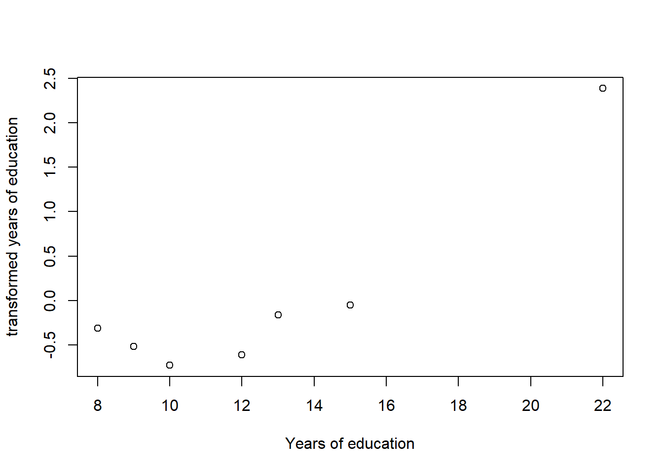

Figure 2: Plots of the response and predictors using acepack

plot(tbtest[,1], acefit$tx[,1], xlab = "Population in region", ylab = "transformed population in region")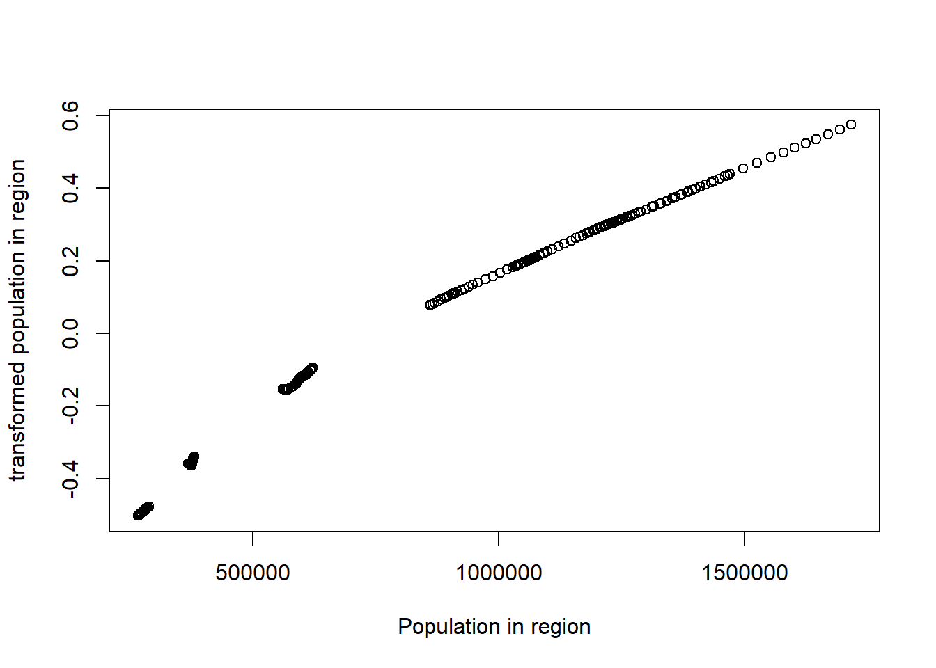

Figure 3: Plots of the response and predictors using acepack

plot(tbtest[,2], acefit$tx[,2], xlab = "# persons with same edulevel, region, year", ylab = "transformed # persons with same edulevel, region, year")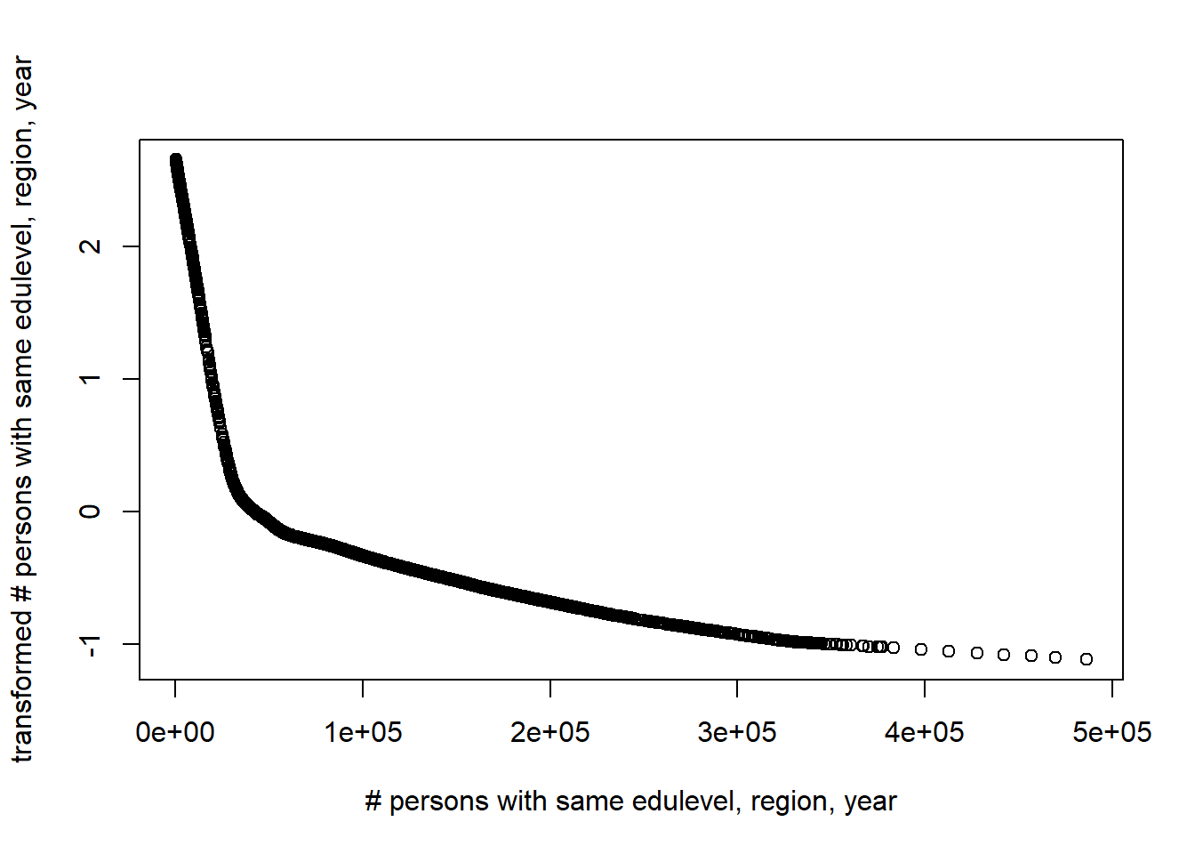

Figure 4: Plots of the response and predictors using acepack

plot(tbtest[,3], acefit$tx[,3], xlab = "Year", ylab = "transformed year")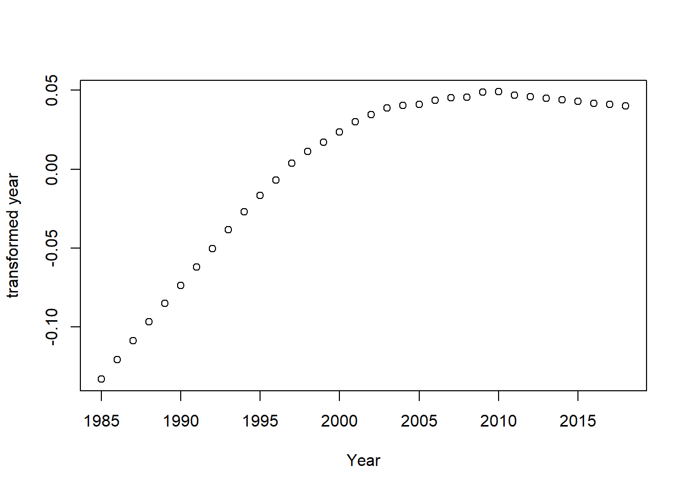

Figure 5: Plots of the response and predictors using acepack

plot(tbtest[,4], acefit$tx[,4], xlab = "Percent women", ylab = "transformed percent women")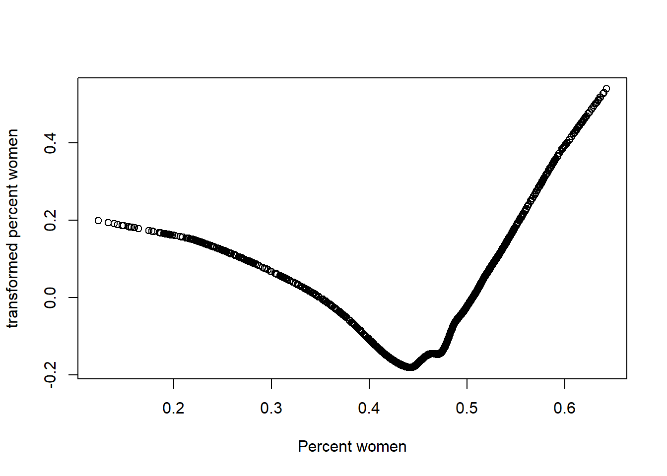

Figure 6: Plots of the response and predictors using acepack

I use MARS to fit hockey-stick functions for the predictors. I do not wish to overfit by using a better approximation at this point. I will include interactions of degree two.

tbtest <- tbnum %>% dplyr::select(eduyears, sum_pop, sum_edu_region_year, year_n, perc_women)

mmod <- earth(eduyears ~ ., data=tbtest, nk = 9, degree = 2)

summary (mmod)

## Call: earth(formula=eduyears~., data=tbtest, degree=2, nk=9)
## 
##                                                       coefficients
## (Intercept)                                               9.930701
## h(37001-sum_edu_region_year)                              0.000380
## h(sum_edu_region_year-37001)                              0.000003
## h(0.492816-perc_women)                                    9.900436
## h(perc_women-0.492816)                                   49.719932
## h(1.32988e+06-sum_pop) * h(37001-sum_edu_region_year)     0.000000
## h(sum_pop-1.32988e+06) * h(37001-sum_edu_region_year)     0.000000
## h(sum_edu_region_year-37001) * h(2004-year_n)            -0.000001
## 
## Selected 8 of 9 terms, and 4 of 4 predictors
## Termination condition: Reached nk 9
## Importance: sum_edu_region_year, perc_women, sum_pop, year_n
## Number of terms at each degree of interaction: 1 4 3
## GCV 3.774465    RSS 86099.37    GRSq 0.8049234    RSq 0.8052222

plot (mmod)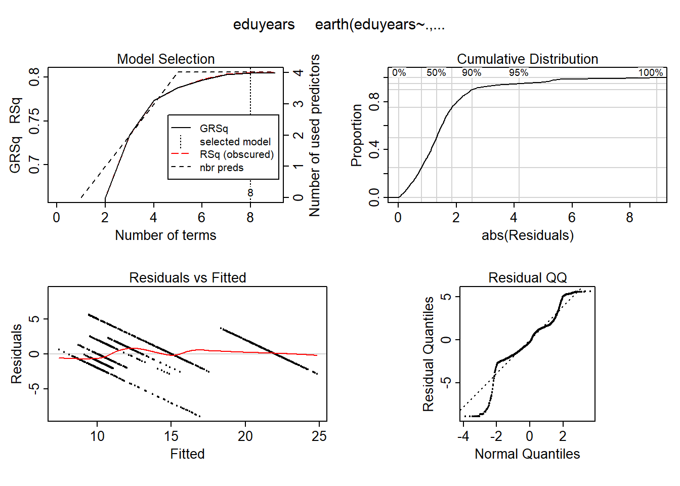

Figure 7: Hockey-stick functions fit with MARS for the predictors, Year 1985 - 2018

plotmo (mmod)

##  plotmo grid:    sum_pop sum_edu_region_year year_n perc_women
##                   740931             90870.5 2001.5  0.4815703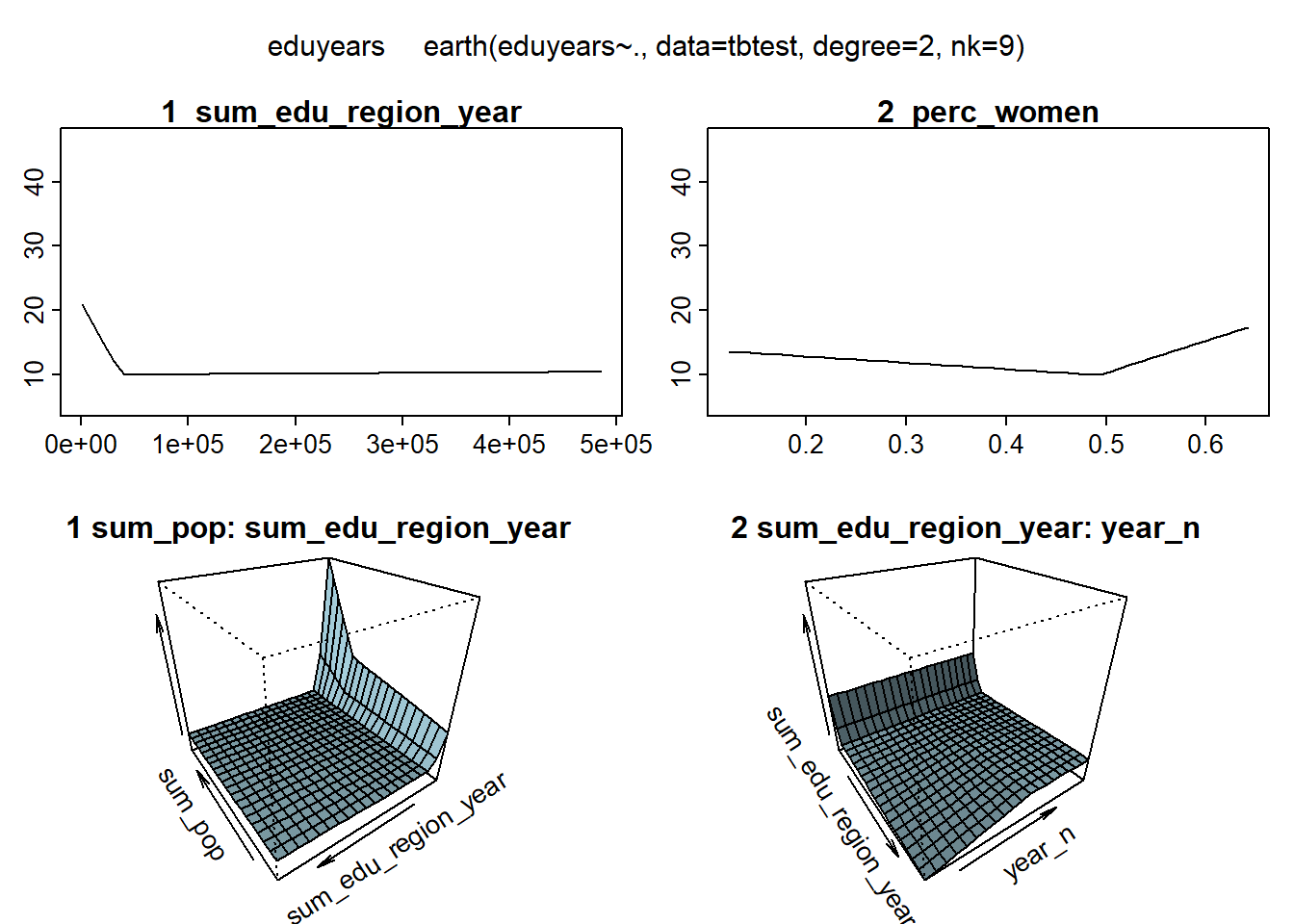

Figure 8: Hockey-stick functions fit with MARS for the predictors, Year 1985 - 2018

model_mmod <- lm (eduyears ~ lspline(sum_edu_region_year, c(37001)) + 
              lspline(perc_women, c(0.492816)) + 
              lspline(sum_pop, c(1.32988e+06)):lspline(sum_edu_region_year, c(37001)) +
              lspline(sum_edu_region_year, c(1.32988e+06)):lspline(year_n, c(2004)), 
            data = tbnum) 

summary (model_mmod)$r.squared

## [1] 0.7792166

anova (model_mmod)

## Analysis of Variance Table
## 
## Response: eduyears
##                                                                        Df
## lspline(sum_edu_region_year, c(37001))                                  2
## lspline(perc_women, c(0.492816))                                        2
## lspline(sum_edu_region_year, c(37001)):lspline(sum_pop, c(1329880))     4
## lspline(sum_edu_region_year, c(1329880)):lspline(year_n, c(2004))       2
## Residuals                                                           22837
##                                                                     Sum Sq
## lspline(sum_edu_region_year, c(37001))                              292982
## lspline(perc_women, c(0.492816))                                     39071
## lspline(sum_edu_region_year, c(37001)):lspline(sum_pop, c(1329880))   9629
## lspline(sum_edu_region_year, c(1329880)):lspline(year_n, c(2004))     2763
## Residuals                                                            97595
##                                                                     Mean Sq
## lspline(sum_edu_region_year, c(37001))                               146491
## lspline(perc_women, c(0.492816))                                      19535
## lspline(sum_edu_region_year, c(37001)):lspline(sum_pop, c(1329880))    2407
## lspline(sum_edu_region_year, c(1329880)):lspline(year_n, c(2004))      1382
## Residuals                                                                 4
##                                                                      F value
## lspline(sum_edu_region_year, c(37001))                              34278.55
## lspline(perc_women, c(0.492816))                                     4571.22
## lspline(sum_edu_region_year, c(37001)):lspline(sum_pop, c(1329880))   563.27
## lspline(sum_edu_region_year, c(1329880)):lspline(year_n, c(2004))     323.30
## Residuals                                                                   
##                                                                        Pr(>F)
## lspline(sum_edu_region_year, c(37001))                              < 2.2e-16
## lspline(perc_women, c(0.492816))                                    < 2.2e-16
## lspline(sum_edu_region_year, c(37001)):lspline(sum_pop, c(1329880)) < 2.2e-16
## lspline(sum_edu_region_year, c(1329880)):lspline(year_n, c(2004))   < 2.2e-16
## Residuals                                                                    
##                                                                        
## lspline(sum_edu_region_year, c(37001))                              ***
## lspline(perc_women, c(0.492816))                                    ***
## lspline(sum_edu_region_year, c(37001)):lspline(sum_pop, c(1329880)) ***
## lspline(sum_edu_region_year, c(1329880)):lspline(year_n, c(2004))   ***
## Residuals                                                              
## ---
## Signif. codes:  0 '***' 0.001 '**' 0.01 '*' 0.05 '.' 0.1 ' ' 1

I will use regsubsets to find the model which minimises the AIC. I will also calculate the Receiver Operating Characteristic (ROC) for the model I find for each level of years of education.

b <- regsubsets (eduyears ~ (lspline(sum_pop, c(1.32988e+06)) + lspline(perc_women, c(0.492816)) + lspline(year_n, c(2004)) + lspline(sum_edu_region_year, c(37001))) * (lspline(sum_pop, c(1.32988e+06)) + lspline(perc_women, c(0.492816)) + lspline(year_n, c(2004)) + lspline(sum_edu_region_year, c(37001))), data = tbnum, nvmax = 20)

rs <- summary(b)
AIC <- 50 * log (rs$rss / 50) + (2:21) * 2
which.min (AIC)

## [1] 9

names (rs$which[9,])[rs$which[9,]]

##  [1] "(Intercept)"                                                              
##  [2] "lspline(sum_pop, c(1329880))1"                                            
##  [3] "lspline(sum_edu_region_year, c(37001))2"                                  
##  [4] "lspline(sum_pop, c(1329880))1:lspline(perc_women, c(0.492816))1"          
##  [5] "lspline(sum_pop, c(1329880))1:lspline(year_n, c(2004))1"                  
##  [6] "lspline(sum_pop, c(1329880))1:lspline(sum_edu_region_year, c(37001))1"    
##  [7] "lspline(perc_women, c(0.492816))1:lspline(year_n, c(2004))1"              
##  [8] "lspline(perc_women, c(0.492816))2:lspline(year_n, c(2004))1"              
##  [9] "lspline(perc_women, c(0.492816))1:lspline(sum_edu_region_year, c(37001))2"
## [10] "lspline(year_n, c(2004))1:lspline(sum_edu_region_year, c(37001))2"

model <- lm(eduyears ~ 
  lspline(sum_pop, c(1329880)) + 
  lspline(sum_edu_region_year, c(37001)) + 
  lspline(sum_pop, c(1329880)):lspline(perc_women, c(0.492816)) +
  lspline(sum_pop, c(1329880)):lspline(year_n, c(2004)) +
  lspline(sum_pop, c(1329880)):lspline(sum_edu_region_year, c(37001)) +
  lspline(perc_women, c(0.492816)):lspline(year_n, c(2004)) +
  lspline(perc_women, c(0.492816)):lspline(sum_edu_region_year, c(37001)) +
  lspline(year_n, c(2004)):lspline(sum_edu_region_year, c(37001)), 
  data = tbnum) 

summary (model)$r.squared

## [1] 0.8455547

anova (model)

## Analysis of Variance Table
## 
## Response: eduyears
##                                                                            Df
## lspline(sum_pop, c(1329880))                                                2
## lspline(sum_edu_region_year, c(37001))                                      2
## lspline(sum_pop, c(1329880)):lspline(perc_women, c(0.492816))               4
## lspline(sum_pop, c(1329880)):lspline(year_n, c(2004))                       4
## lspline(sum_pop, c(1329880)):lspline(sum_edu_region_year, c(37001))         4
## lspline(perc_women, c(0.492816)):lspline(year_n, c(2004))                   4
## lspline(sum_edu_region_year, c(37001)):lspline(perc_women, c(0.492816))     4
## lspline(sum_edu_region_year, c(37001)):lspline(year_n, c(2004))             4
## Residuals                                                               22819
##                                                                         Sum Sq
## lspline(sum_pop, c(1329880))                                                 0
## lspline(sum_edu_region_year, c(37001))                                  306779
## lspline(sum_pop, c(1329880)):lspline(perc_women, c(0.492816))            35378
## lspline(sum_pop, c(1329880)):lspline(year_n, c(2004))                      775
## lspline(sum_pop, c(1329880)):lspline(sum_edu_region_year, c(37001))       7224
## lspline(perc_women, c(0.492816)):lspline(year_n, c(2004))                 8932
## lspline(sum_edu_region_year, c(37001)):lspline(perc_women, c(0.492816))   6979
## lspline(sum_edu_region_year, c(37001)):lspline(year_n, c(2004))           7700
## Residuals                                                                68271
##                                                                         Mean Sq
## lspline(sum_pop, c(1329880))                                                  0
## lspline(sum_edu_region_year, c(37001))                                   153389
## lspline(sum_pop, c(1329880)):lspline(perc_women, c(0.492816))              8844
## lspline(sum_pop, c(1329880)):lspline(year_n, c(2004))                       194
## lspline(sum_pop, c(1329880)):lspline(sum_edu_region_year, c(37001))        1806
## lspline(perc_women, c(0.492816)):lspline(year_n, c(2004))                  2233
## lspline(sum_edu_region_year, c(37001)):lspline(perc_women, c(0.492816))    1745
## lspline(sum_edu_region_year, c(37001)):lspline(year_n, c(2004))            1925
## Residuals                                                                     3
##                                                                          F value
## lspline(sum_pop, c(1329880))                                                0.00
## lspline(sum_edu_region_year, c(37001))                                  51269.26
## lspline(sum_pop, c(1329880)):lspline(perc_women, c(0.492816))            2956.20
## lspline(sum_pop, c(1329880)):lspline(year_n, c(2004))                      64.80
## lspline(sum_pop, c(1329880)):lspline(sum_edu_region_year, c(37001))       603.67
## lspline(perc_women, c(0.492816)):lspline(year_n, c(2004))                 746.37
## lspline(sum_edu_region_year, c(37001)):lspline(perc_women, c(0.492816))   583.19
## lspline(sum_edu_region_year, c(37001)):lspline(year_n, c(2004))           643.44
## Residuals                                                                       
##                                                                         Pr(>F)
## lspline(sum_pop, c(1329880))                                                 1
## lspline(sum_edu_region_year, c(37001))                                  <2e-16
## lspline(sum_pop, c(1329880)):lspline(perc_women, c(0.492816))           <2e-16
## lspline(sum_pop, c(1329880)):lspline(year_n, c(2004))                   <2e-16
## lspline(sum_pop, c(1329880)):lspline(sum_edu_region_year, c(37001))     <2e-16
## lspline(perc_women, c(0.492816)):lspline(year_n, c(2004))               <2e-16
## lspline(sum_edu_region_year, c(37001)):lspline(perc_women, c(0.492816)) <2e-16
## lspline(sum_edu_region_year, c(37001)):lspline(year_n, c(2004))         <2e-16
## Residuals                                                                     
##                                                                            
## lspline(sum_pop, c(1329880))                                               
## lspline(sum_edu_region_year, c(37001))                                  ***
## lspline(sum_pop, c(1329880)):lspline(perc_women, c(0.492816))           ***
## lspline(sum_pop, c(1329880)):lspline(year_n, c(2004))                   ***
## lspline(sum_pop, c(1329880)):lspline(sum_edu_region_year, c(37001))     ***
## lspline(perc_women, c(0.492816)):lspline(year_n, c(2004))               ***
## lspline(sum_edu_region_year, c(37001)):lspline(perc_women, c(0.492816)) ***
## lspline(sum_edu_region_year, c(37001)):lspline(year_n, c(2004))         ***
## Residuals                                                                  
## ---
## Signif. codes:  0 '***' 0.001 '**' 0.01 '*' 0.05 '.' 0.1 ' ' 1

plot (model)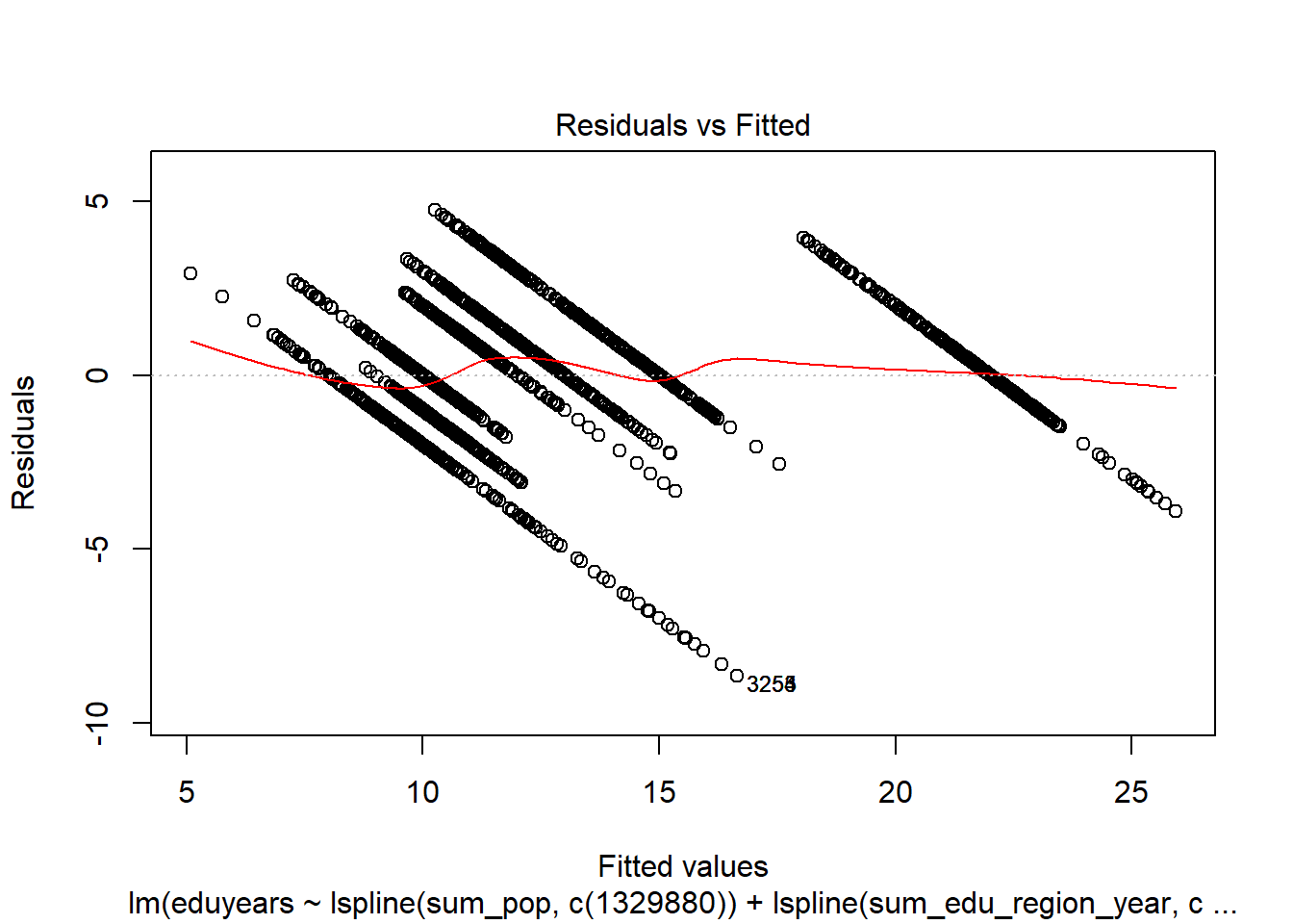

Figure 9: Find the model that minimises the AIC, Year 1985 - 2018

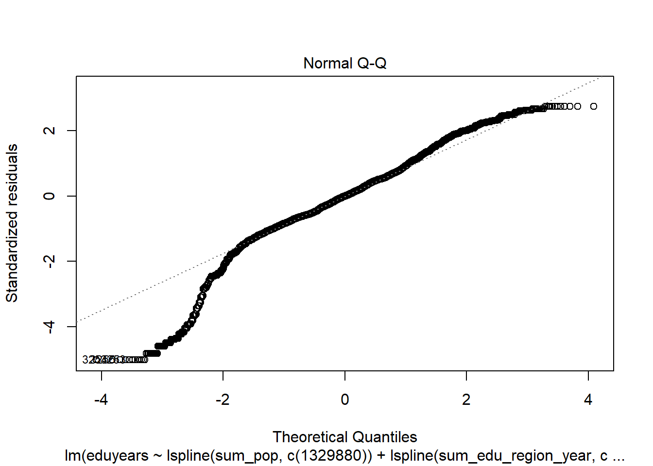
Figure 10: Find the model that minimises the AIC, Year 1985 - 2018

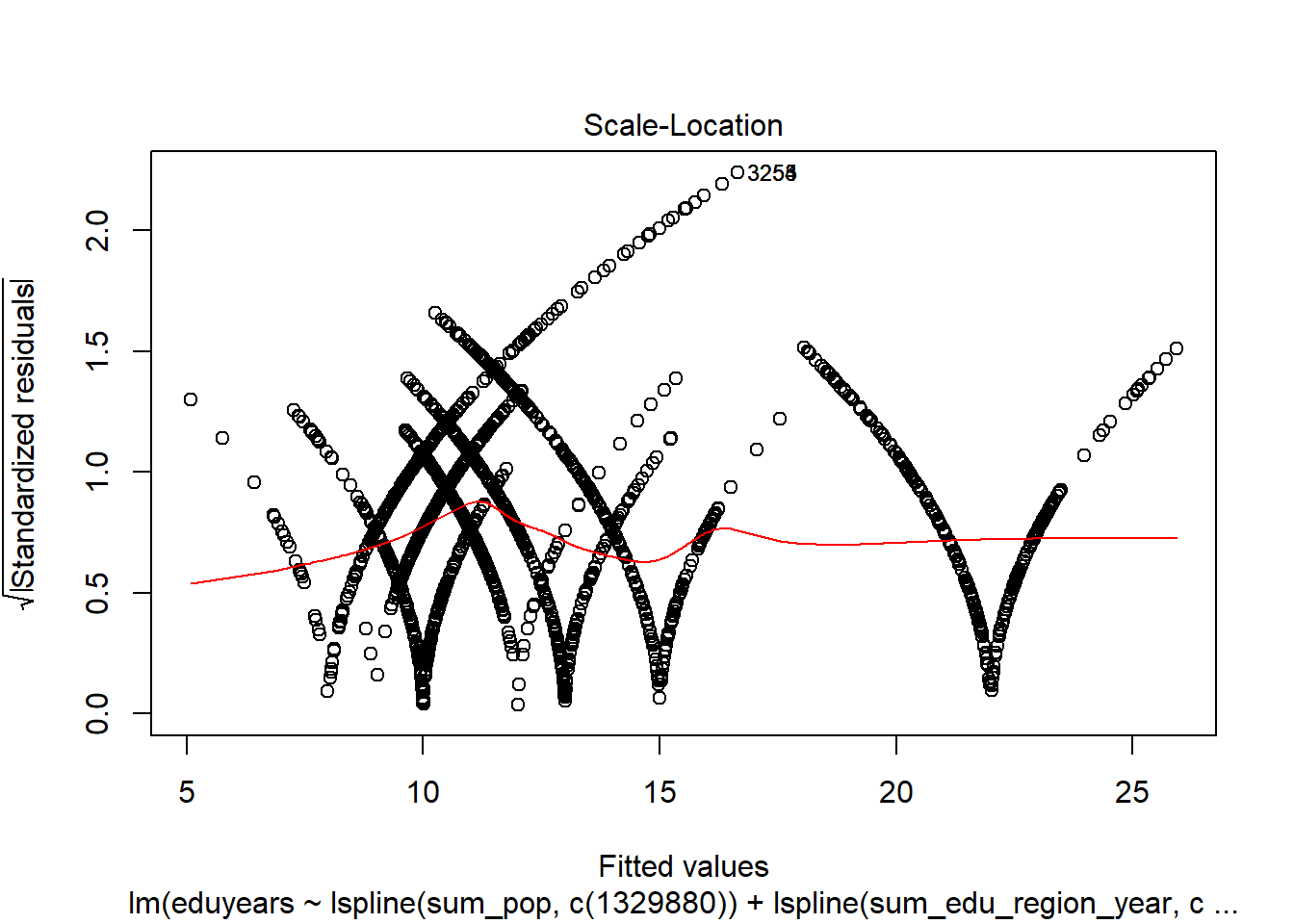
Figure 11: Find the model that minimises the AIC, Year 1985 - 2018

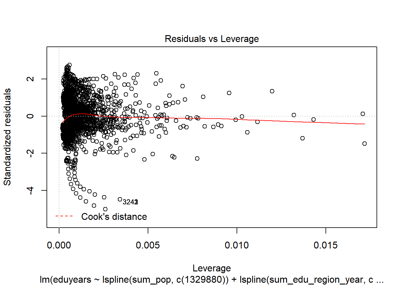
Figure 12: Find the model that minimises the AIC, Year 1985 - 2018

tbnumpred <- bind_cols(tbnum, as_tibble(predict(model, tbnum, interval = "confidence")))

suppressWarnings(multiclass.roc(tbnumpred$eduyears, tbnumpred$fit))

## Setting direction: controls < cases
## Setting direction: controls < cases
## Setting direction: controls < cases
## Setting direction: controls < cases
## Setting direction: controls < cases
## Setting direction: controls < cases

## Setting direction: controls > cases

## Setting direction: controls < cases
## Setting direction: controls < cases
## Setting direction: controls < cases
## Setting direction: controls < cases
## Setting direction: controls < cases
## Setting direction: controls < cases
## Setting direction: controls < cases
## Setting direction: controls < cases
## Setting direction: controls < cases
## Setting direction: controls < cases
## Setting direction: controls < cases
## Setting direction: controls < cases
## Setting direction: controls < cases
## Setting direction: controls < cases

## 
## Call:
## multiclass.roc.default(response = tbnumpred$eduyears, predictor = tbnumpred$fit)
## 
## Data: tbnumpred$fit with 7 levels of tbnumpred$eduyears: 8, 9, 10, 12, 13, 15, 22.
## Multi-class area under the curve: 0.8743

There are a few things I would like to investigate to improve the credibility of the analysis. First, the study is a longitudinal study. A great proportion of people is measured each year. The majority of the people in the region remains in the region from year to year. I will assume that each birthyear and each region is a group and set them as random effects and the rest of the predictors as fixed effects. I use the mean age in each age group as the year of birth.

temp <- tbnum %>% mutate(yob = year_n - age_n) %>% mutate(region = tbnum$region)

mmodel <- lmer(eduyears ~
  lspline(sum_pop, c(1329880)) + 
  lspline(sum_edu_region_year, c(37001)) + 
  lspline(sum_pop, c(1329880)):lspline(perc_women, c(0.492816)) +
  lspline(sum_pop, c(1329880)):lspline(year_n, c(2004)) +
  lspline(sum_pop, c(1329880)):lspline(sum_edu_region_year, c(37001)) +
  lspline(perc_women, c(0.492816)):lspline(year_n, c(2004)) +
  lspline(perc_women, c(0.492816)):lspline(sum_edu_region_year, c(37001)) +
  lspline(year_n, c(2004)):lspline(sum_edu_region_year, c(37001)) +
  (1|yob) + 
  (1|region),
  data = temp)

## Warning: Some predictor variables are on very different scales: consider
## rescaling

## boundary (singular) fit: see ?isSingular

plot(mmodel)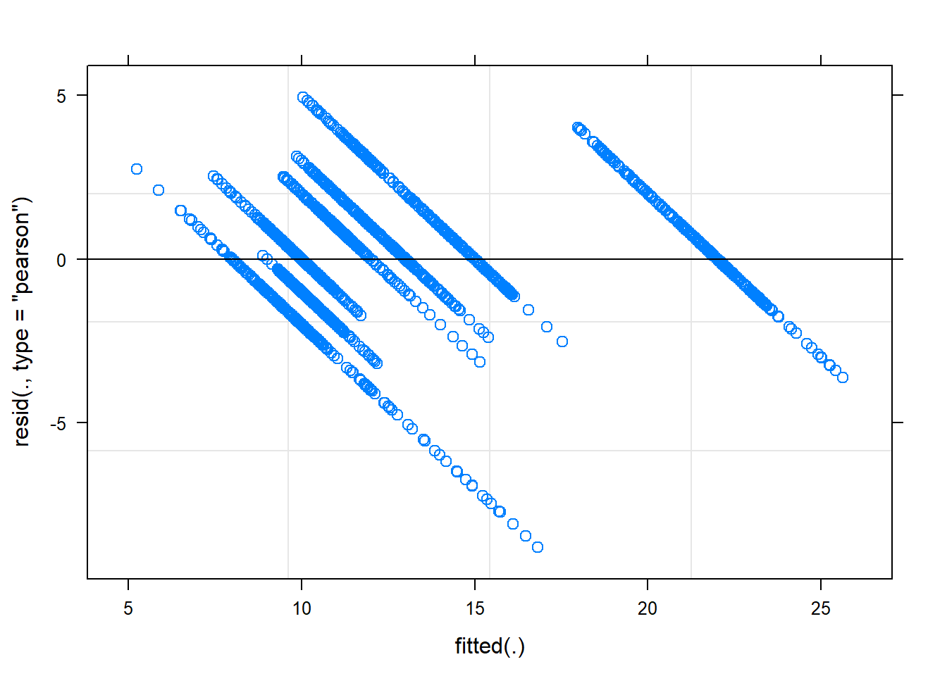

Figure 13: A diagnostic plot of the model with random effects components

qqnorm (residuals(mmodel), main="")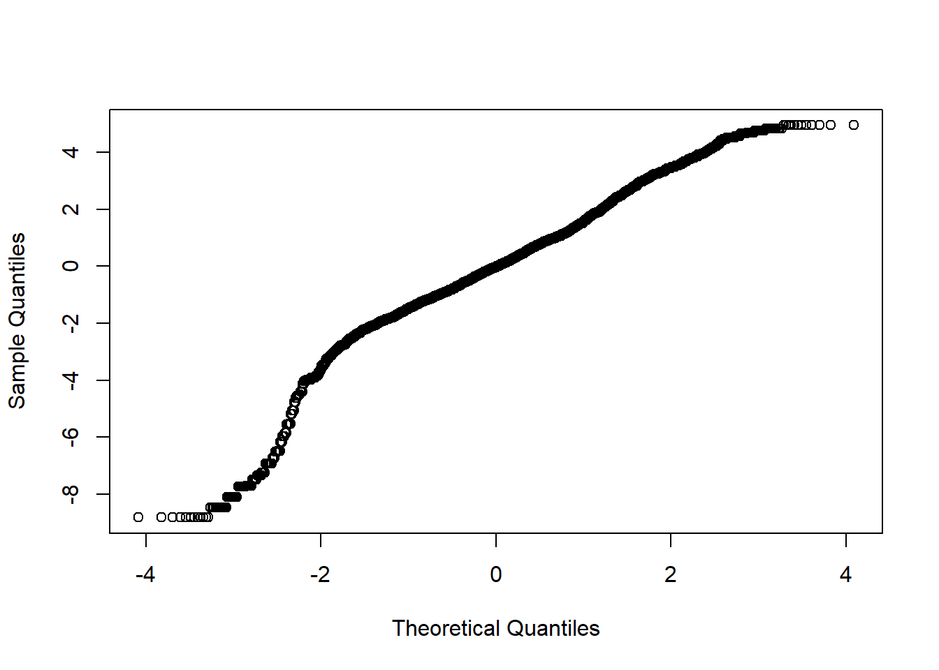

Figure 14: A diagnostic plot of the model with random effects components

summary (mmodel)

## Linear mixed model fit by REML ['lmerMod']
## Formula: 
## eduyears ~ lspline(sum_pop, c(1329880)) + lspline(sum_edu_region_year,  
##     c(37001)) + lspline(sum_pop, c(1329880)):lspline(perc_women,  
##     c(0.492816)) + lspline(sum_pop, c(1329880)):lspline(year_n,  
##     c(2004)) + lspline(sum_pop, c(1329880)):lspline(sum_edu_region_year,  
##     c(37001)) + lspline(perc_women, c(0.492816)):lspline(year_n,  
##     c(2004)) + lspline(perc_women, c(0.492816)):lspline(sum_edu_region_year,  
##     c(37001)) + lspline(year_n, c(2004)):lspline(sum_edu_region_year,  
##     c(37001)) + (1 | yob) + (1 | region)
##    Data: temp
## 
## REML criterion at convergence: 90514.4
## 
## Scaled residuals: 
##     Min      1Q  Median      3Q     Max 
## -5.1175 -0.5978 -0.0137  0.5766  2.8735 
## 
## Random effects:
##  Groups   Name        Variance Std.Dev.
##  yob      (Intercept) 0.000    0.000   
##  region   (Intercept) 1.115    1.056   
##  Residual             2.970    1.723   
## Number of obs: 22848, groups:  yob, 108; region, 8
## 
## Fixed effects:
##                                                                             Estimate
## (Intercept)                                                                2.516e+01
## lspline(sum_pop, c(1329880))1                                              1.514e-04
## lspline(sum_pop, c(1329880))2                                              2.912e-03
## lspline(sum_edu_region_year, c(37001))1                                    2.314e-03
## lspline(sum_edu_region_year, c(37001))2                                   -2.288e-03
## lspline(sum_pop, c(1329880))1:lspline(perc_women, c(0.492816))1            5.502e-05
## lspline(sum_pop, c(1329880))2:lspline(perc_women, c(0.492816))1            7.840e-05
## lspline(sum_pop, c(1329880))1:lspline(perc_women, c(0.492816))2           -2.061e-05
## lspline(sum_pop, c(1329880))2:lspline(perc_women, c(0.492816))2            1.467e-05
## lspline(sum_pop, c(1329880))1:lspline(year_n, c(2004))1                   -7.788e-08
## lspline(sum_pop, c(1329880))2:lspline(year_n, c(2004))1                   -1.428e-06
## lspline(sum_pop, c(1329880))1:lspline(year_n, c(2004))2                   -3.009e-07
## lspline(sum_pop, c(1329880))2:lspline(year_n, c(2004))2                    1.430e-07
## lspline(sum_pop, c(1329880))1:lspline(sum_edu_region_year, c(37001))1     -4.707e-10
## lspline(sum_pop, c(1329880))2:lspline(sum_edu_region_year, c(37001))1     -2.387e-09
## lspline(sum_pop, c(1329880))1:lspline(sum_edu_region_year, c(37001))2      2.554e-13
## lspline(sum_pop, c(1329880))2:lspline(sum_edu_region_year, c(37001))2      1.137e-12
## lspline(perc_women, c(0.492816))1:lspline(year_n, c(2004))1               -1.659e-02
## lspline(perc_women, c(0.492816))2:lspline(year_n, c(2004))1                3.580e-02
## lspline(perc_women, c(0.492816))1:lspline(year_n, c(2004))2                3.888e-01
## lspline(perc_women, c(0.492816))2:lspline(year_n, c(2004))2               -1.008e+00
## lspline(sum_edu_region_year, c(37001))1:lspline(perc_women, c(0.492816))1  9.201e-05
## lspline(sum_edu_region_year, c(37001))2:lspline(perc_women, c(0.492816))1 -4.149e-04
## lspline(sum_edu_region_year, c(37001))1:lspline(perc_women, c(0.492816))2 -1.441e-04
## lspline(sum_edu_region_year, c(37001))2:lspline(perc_women, c(0.492816))2  1.086e-04
## lspline(sum_edu_region_year, c(37001))1:lspline(year_n, c(2004))1         -1.211e-06
## lspline(sum_edu_region_year, c(37001))2:lspline(year_n, c(2004))1          1.240e-06
## lspline(sum_edu_region_year, c(37001))1:lspline(year_n, c(2004))2         -2.615e-06
## lspline(sum_edu_region_year, c(37001))2:lspline(year_n, c(2004))2          1.146e-06
##                                                                           Std. Error
## (Intercept)                                                                6.548e-01
## lspline(sum_pop, c(1329880))1                                              1.494e-05
## lspline(sum_pop, c(1329880))2                                              6.394e-03
## lspline(sum_edu_region_year, c(37001))1                                    3.150e-04
## lspline(sum_edu_region_year, c(37001))2                                    7.229e-05
## lspline(sum_pop, c(1329880))1:lspline(perc_women, c(0.492816))1            1.344e-06
## lspline(sum_pop, c(1329880))2:lspline(perc_women, c(0.492816))1            1.213e-05
## lspline(sum_pop, c(1329880))1:lspline(perc_women, c(0.492816))2            2.853e-06
## lspline(sum_pop, c(1329880))2:lspline(perc_women, c(0.492816))2            1.540e-05
## lspline(sum_pop, c(1329880))1:lspline(year_n, c(2004))1                    7.362e-09
## lspline(sum_pop, c(1329880))2:lspline(year_n, c(2004))1                    3.191e-06
## lspline(sum_pop, c(1329880))1:lspline(year_n, c(2004))2                    1.349e-08
## lspline(sum_pop, c(1329880))2:lspline(year_n, c(2004))2                    7.352e-08
## lspline(sum_pop, c(1329880))1:lspline(sum_edu_region_year, c(37001))1      9.596e-12
## lspline(sum_pop, c(1329880))2:lspline(sum_edu_region_year, c(37001))1      8.271e-11
## lspline(sum_pop, c(1329880))1:lspline(sum_edu_region_year, c(37001))2      7.991e-13
## lspline(sum_pop, c(1329880))2:lspline(sum_edu_region_year, c(37001))2      2.836e-12
## lspline(perc_women, c(0.492816))1:lspline(year_n, c(2004))1                4.545e-04
## lspline(perc_women, c(0.492816))2:lspline(year_n, c(2004))1                4.504e-03
## lspline(perc_women, c(0.492816))1:lspline(year_n, c(2004))2                3.671e-02
## lspline(perc_women, c(0.492816))2:lspline(year_n, c(2004))2                9.737e-02
## lspline(sum_edu_region_year, c(37001))1:lspline(perc_women, c(0.492816))1  2.688e-05
## lspline(sum_edu_region_year, c(37001))2:lspline(perc_women, c(0.492816))1  1.117e-05
## lspline(sum_edu_region_year, c(37001))1:lspline(perc_women, c(0.492816))2  2.526e-04
## lspline(sum_edu_region_year, c(37001))2:lspline(perc_women, c(0.492816))2  1.429e-05
## lspline(sum_edu_region_year, c(37001))1:lspline(year_n, c(2004))1          1.586e-07
## lspline(sum_edu_region_year, c(37001))2:lspline(year_n, c(2004))1          3.623e-08
## lspline(sum_edu_region_year, c(37001))1:lspline(year_n, c(2004))2          4.441e-07
## lspline(sum_edu_region_year, c(37001))2:lspline(year_n, c(2004))2          6.085e-08
##                                                                           t value
## (Intercept)                                                                38.420
## lspline(sum_pop, c(1329880))1                                              10.137
## lspline(sum_pop, c(1329880))2                                               0.455
## lspline(sum_edu_region_year, c(37001))1                                     7.345
## lspline(sum_edu_region_year, c(37001))2                                   -31.645
## lspline(sum_pop, c(1329880))1:lspline(perc_women, c(0.492816))1            40.921
## lspline(sum_pop, c(1329880))2:lspline(perc_women, c(0.492816))1             6.463
## lspline(sum_pop, c(1329880))1:lspline(perc_women, c(0.492816))2            -7.226
## lspline(sum_pop, c(1329880))2:lspline(perc_women, c(0.492816))2             0.952
## lspline(sum_pop, c(1329880))1:lspline(year_n, c(2004))1                   -10.579
## lspline(sum_pop, c(1329880))2:lspline(year_n, c(2004))1                    -0.448
## lspline(sum_pop, c(1329880))1:lspline(year_n, c(2004))2                   -22.303
## lspline(sum_pop, c(1329880))2:lspline(year_n, c(2004))2                     1.945
## lspline(sum_pop, c(1329880))1:lspline(sum_edu_region_year, c(37001))1     -49.052
## lspline(sum_pop, c(1329880))2:lspline(sum_edu_region_year, c(37001))1     -28.855
## lspline(sum_pop, c(1329880))1:lspline(sum_edu_region_year, c(37001))2       0.320
## lspline(sum_pop, c(1329880))2:lspline(sum_edu_region_year, c(37001))2       0.401
## lspline(perc_women, c(0.492816))1:lspline(year_n, c(2004))1               -36.497
## lspline(perc_women, c(0.492816))2:lspline(year_n, c(2004))1                 7.949
## lspline(perc_women, c(0.492816))1:lspline(year_n, c(2004))2                10.593
## lspline(perc_women, c(0.492816))2:lspline(year_n, c(2004))2               -10.350
## lspline(sum_edu_region_year, c(37001))1:lspline(perc_women, c(0.492816))1   3.423
## lspline(sum_edu_region_year, c(37001))2:lspline(perc_women, c(0.492816))1 -37.150
## lspline(sum_edu_region_year, c(37001))1:lspline(perc_women, c(0.492816))2  -0.571
## lspline(sum_edu_region_year, c(37001))2:lspline(perc_women, c(0.492816))2   7.602
## lspline(sum_edu_region_year, c(37001))1:lspline(year_n, c(2004))1          -7.639
## lspline(sum_edu_region_year, c(37001))2:lspline(year_n, c(2004))1          34.226
## lspline(sum_edu_region_year, c(37001))1:lspline(year_n, c(2004))2          -5.887
## lspline(sum_edu_region_year, c(37001))2:lspline(year_n, c(2004))2          18.833

## 
## Correlation matrix not shown by default, as p = 29 > 12.
## Use print(x, correlation=TRUE)  or
##     vcov(x)        if you need it

## fit warnings:
## Some predictor variables are on very different scales: consider rescaling
## convergence code: 0
## boundary (singular) fit: see ?isSingular

anova (mmodel)

## Analysis of Variance Table
##                                                                         Df
## lspline(sum_pop, c(1329880))                                             2
## lspline(sum_edu_region_year, c(37001))                                   2
## lspline(sum_pop, c(1329880)):lspline(perc_women, c(0.492816))            4
## lspline(sum_pop, c(1329880)):lspline(year_n, c(2004))                    4
## lspline(sum_pop, c(1329880)):lspline(sum_edu_region_year, c(37001))      4
## lspline(perc_women, c(0.492816)):lspline(year_n, c(2004))                4
## lspline(sum_edu_region_year, c(37001)):lspline(perc_women, c(0.492816))  4
## lspline(sum_edu_region_year, c(37001)):lspline(year_n, c(2004))          4
##                                                                         Sum Sq
## lspline(sum_pop, c(1329880))                                                 0
## lspline(sum_edu_region_year, c(37001))                                  308190
## lspline(sum_pop, c(1329880)):lspline(perc_women, c(0.492816))            35415
## lspline(sum_pop, c(1329880)):lspline(year_n, c(2004))                      589
## lspline(sum_pop, c(1329880)):lspline(sum_edu_region_year, c(37001))       7737
## lspline(perc_women, c(0.492816)):lspline(year_n, c(2004))                 8202
## lspline(sum_edu_region_year, c(37001)):lspline(perc_women, c(0.492816))   7316
## lspline(sum_edu_region_year, c(37001)):lspline(year_n, c(2004))           6809
##                                                                         Mean Sq
## lspline(sum_pop, c(1329880))                                                  0
## lspline(sum_edu_region_year, c(37001))                                   154095
## lspline(sum_pop, c(1329880)):lspline(perc_women, c(0.492816))              8854
## lspline(sum_pop, c(1329880)):lspline(year_n, c(2004))                       147
## lspline(sum_pop, c(1329880)):lspline(sum_edu_region_year, c(37001))        1934
## lspline(perc_women, c(0.492816)):lspline(year_n, c(2004))                  2051
## lspline(sum_edu_region_year, c(37001)):lspline(perc_women, c(0.492816))    1829
## lspline(sum_edu_region_year, c(37001)):lspline(year_n, c(2004))            1702
##                                                                           F value
## lspline(sum_pop, c(1329880))                                                0.000
## lspline(sum_edu_region_year, c(37001))                                  51879.188
## lspline(sum_pop, c(1329880)):lspline(perc_women, c(0.492816))            2980.805
## lspline(sum_pop, c(1329880)):lspline(year_n, c(2004))                      49.613
## lspline(sum_pop, c(1329880)):lspline(sum_edu_region_year, c(37001))       651.234
## lspline(perc_women, c(0.492816)):lspline(year_n, c(2004))                 690.377
## lspline(sum_edu_region_year, c(37001)):lspline(perc_women, c(0.492816))   615.763
## lspline(sum_edu_region_year, c(37001)):lspline(year_n, c(2004))           573.138

tbnumpred <- bind_cols(temp, as_tibble(predict(mmodel, temp, interval = "confidence")))

## Warning in predict.merMod(mmodel, temp, interval = "confidence"): unused
## arguments ignored

## Warning: Calling `as_tibble()` on a vector is discouraged, because the behavior is likely to change in the future. Use `tibble::enframe(name = NULL)` instead.
## This warning is displayed once per session.

suppressWarnings (multiclass.roc (tbnumpred$eduyears, tbnumpred$value))

## Setting direction: controls < cases

## Setting direction: controls < cases
## Setting direction: controls < cases
## Setting direction: controls < cases
## Setting direction: controls < cases
## Setting direction: controls < cases

## Setting direction: controls > cases

## Setting direction: controls < cases
## Setting direction: controls < cases
## Setting direction: controls < cases
## Setting direction: controls < cases
## Setting direction: controls < cases
## Setting direction: controls < cases
## Setting direction: controls < cases
## Setting direction: controls < cases
## Setting direction: controls < cases
## Setting direction: controls < cases
## Setting direction: controls < cases
## Setting direction: controls < cases
## Setting direction: controls < cases
## Setting direction: controls < cases

## 
## Call:
## multiclass.roc.default(response = tbnumpred$eduyears, predictor = tbnumpred$value)
## 
## Data: tbnumpred$value with 7 levels of tbnumpred$eduyears: 8, 9, 10, 12, 13, 15, 22.
## Multi-class area under the curve: 0.8754

Another problem could be that the response variable is limited in its range. To get more insight about this issue we could model with Poisson regression.

pmodel <- glm(eduyears ~ 
  lspline(sum_pop, c(1329880)) + 
  lspline(sum_edu_region_year, c(37001)) + 
  lspline(sum_pop, c(1329880)):lspline(perc_women, c(0.492816)) +
  lspline(sum_pop, c(1329880)):lspline(year_n, c(2004)) +
  lspline(sum_pop, c(1329880)):lspline(sum_edu_region_year, c(37001)) +
  lspline(perc_women, c(0.492816)):lspline(year_n, c(2004)) +
  lspline(perc_women, c(0.492816)):lspline(sum_edu_region_year, c(37001)) +
  lspline(year_n, c(2004)):lspline(sum_edu_region_year, c(37001)),
  family = poisson,
  data = tbnum) 

plot (pmodel)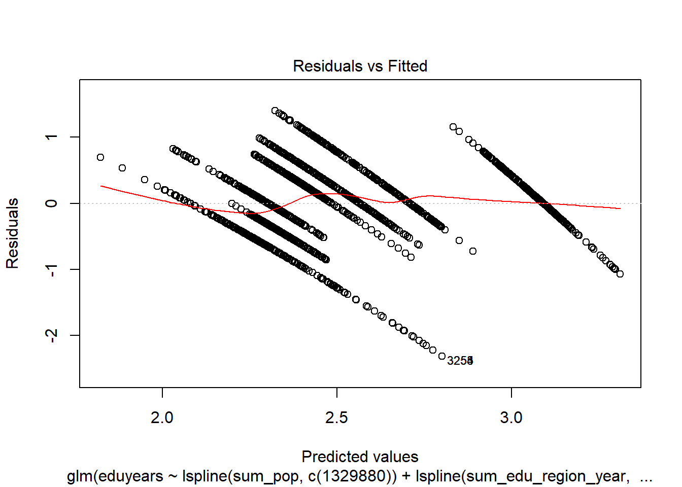

Figure 15: A diagnostic plot of Poisson regression

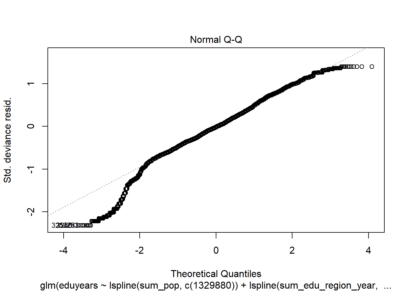
Figure 16: A diagnostic plot of Poisson regression

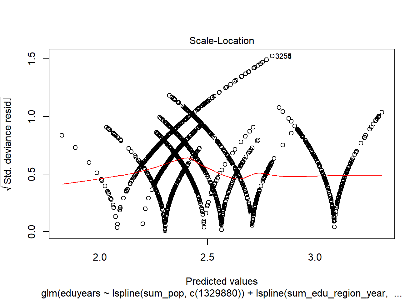
Figure 17: A diagnostic plot of Poisson regression

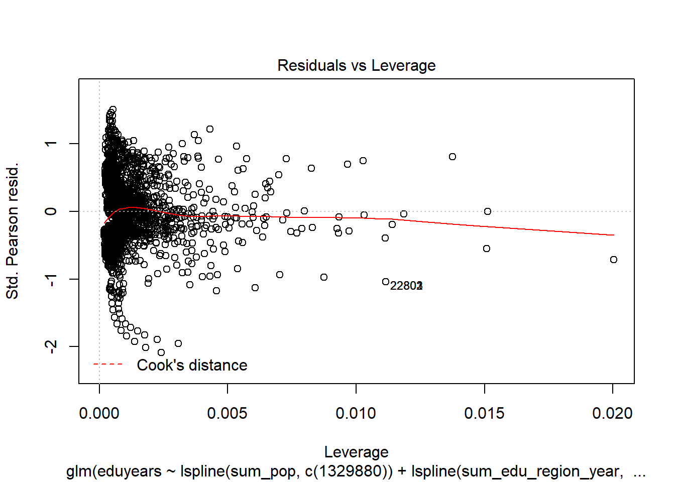
Figure 18: A diagnostic plot of Poisson regression

tbnumpred <- bind_cols(tbnum, as_tibble(predict(pmodel, tbnum, interval = "confidence")))

suppressWarnings (multiclass.roc (tbnumpred$eduyears, tbnumpred$value))

## Setting direction: controls < cases
## Setting direction: controls < cases
## Setting direction: controls < cases
## Setting direction: controls < cases
## Setting direction: controls < cases
## Setting direction: controls < cases

## Setting direction: controls > cases

## Setting direction: controls < cases
## Setting direction: controls < cases
## Setting direction: controls < cases
## Setting direction: controls < cases
## Setting direction: controls < cases
## Setting direction: controls < cases
## Setting direction: controls < cases
## Setting direction: controls < cases
## Setting direction: controls < cases
## Setting direction: controls < cases
## Setting direction: controls < cases
## Setting direction: controls < cases
## Setting direction: controls < cases
## Setting direction: controls < cases

## 
## Call:
## multiclass.roc.default(response = tbnumpred$eduyears, predictor = tbnumpred$value)
## 
## Data: tbnumpred$value with 7 levels of tbnumpred$eduyears: 8, 9, 10, 12, 13, 15, 22.
## Multi-class area under the curve: 0.8716

summary (pmodel)

## 
## Call:
## glm(formula = eduyears ~ lspline(sum_pop, c(1329880)) + lspline(sum_edu_region_year, 
##     c(37001)) + lspline(sum_pop, c(1329880)):lspline(perc_women, 
##     c(0.492816)) + lspline(sum_pop, c(1329880)):lspline(year_n, 
##     c(2004)) + lspline(sum_pop, c(1329880)):lspline(sum_edu_region_year, 
##     c(37001)) + lspline(perc_women, c(0.492816)):lspline(year_n, 
##     c(2004)) + lspline(perc_women, c(0.492816)):lspline(sum_edu_region_year, 
##     c(37001)) + lspline(year_n, c(2004)):lspline(sum_edu_region_year, 
##     c(37001)), family = poisson, data = tbnum)
## 
## Deviance Residuals: 
##      Min        1Q    Median        3Q       Max  
## -2.32031  -0.33091  -0.01716   0.30301   1.40215  
## 
## Coefficients:
##                                                                             Estimate
## (Intercept)                                                                3.403e+00
## lspline(sum_pop, c(1329880))1                                              5.825e-06
## lspline(sum_pop, c(1329880))2                                             -8.868e-05
## lspline(sum_edu_region_year, c(37001))1                                    3.722e-04
## lspline(sum_edu_region_year, c(37001))2                                   -2.310e-04
## lspline(sum_pop, c(1329880))1:lspline(perc_women, c(0.492816))1            3.838e-06
## lspline(sum_pop, c(1329880))2:lspline(perc_women, c(0.492816))1            8.103e-06
## lspline(sum_pop, c(1329880))1:lspline(perc_women, c(0.492816))2           -2.276e-06
## lspline(sum_pop, c(1329880))2:lspline(perc_women, c(0.492816))2           -3.732e-06
## lspline(sum_pop, c(1329880))1:lspline(year_n, c(2004))1                   -3.188e-09
## lspline(sum_pop, c(1329880))2:lspline(year_n, c(2004))1                    4.535e-08
## lspline(sum_pop, c(1329880))1:lspline(year_n, c(2004))2                   -2.600e-08
## lspline(sum_pop, c(1329880))2:lspline(year_n, c(2004))2                    1.616e-08
## lspline(sum_pop, c(1329880))1:lspline(sum_edu_region_year, c(37001))1     -2.870e-11
## lspline(sum_pop, c(1329880))2:lspline(sum_edu_region_year, c(37001))1     -1.718e-10
## lspline(sum_pop, c(1329880))1:lspline(sum_edu_region_year, c(37001))2     -2.527e-13
## lspline(sum_pop, c(1329880))2:lspline(sum_edu_region_year, c(37001))2     -2.193e-14
## lspline(perc_women, c(0.492816))1:lspline(year_n, c(2004))1               -9.758e-04
## lspline(perc_women, c(0.492816))2:lspline(year_n, c(2004))1                2.556e-03
## lspline(perc_women, c(0.492816))1:lspline(year_n, c(2004))2                3.188e-02
## lspline(perc_women, c(0.492816))2:lspline(year_n, c(2004))2               -1.221e-01
## lspline(sum_edu_region_year, c(37001))1:lspline(perc_women, c(0.492816))1 -1.020e-05
## lspline(sum_edu_region_year, c(37001))2:lspline(perc_women, c(0.492816))1 -2.991e-05
## lspline(sum_edu_region_year, c(37001))1:lspline(perc_women, c(0.492816))2  1.916e-05
## lspline(sum_edu_region_year, c(37001))2:lspline(perc_women, c(0.492816))2  1.271e-05
## lspline(sum_edu_region_year, c(37001))1:lspline(year_n, c(2004))1         -1.874e-07
## lspline(sum_edu_region_year, c(37001))2:lspline(year_n, c(2004))1          1.224e-07
## lspline(sum_edu_region_year, c(37001))1:lspline(year_n, c(2004))2         -1.952e-07
## lspline(sum_edu_region_year, c(37001))2:lspline(year_n, c(2004))2          1.122e-07
##                                                                           Std. Error
## (Intercept)                                                                3.236e-02
## lspline(sum_pop, c(1329880))1                                              1.792e-06
## lspline(sum_pop, c(1329880))2                                              9.916e-04
## lspline(sum_edu_region_year, c(37001))1                                    4.837e-05
## lspline(sum_edu_region_year, c(37001))2                                    1.222e-05
## lspline(sum_pop, c(1329880))1:lspline(perc_women, c(0.492816))1            1.962e-07
## lspline(sum_pop, c(1329880))2:lspline(perc_women, c(0.492816))1            2.131e-06
## lspline(sum_pop, c(1329880))1:lspline(perc_women, c(0.492816))2            4.682e-07
## lspline(sum_pop, c(1329880))2:lspline(perc_women, c(0.492816))2            2.516e-06
## lspline(sum_pop, c(1329880))1:lspline(year_n, c(2004))1                    9.022e-10
## lspline(sum_pop, c(1329880))2:lspline(year_n, c(2004))1                    4.948e-07
## lspline(sum_pop, c(1329880))1:lspline(year_n, c(2004))2                    1.917e-09
## lspline(sum_pop, c(1329880))2:lspline(year_n, c(2004))2                    1.155e-08
## lspline(sum_pop, c(1329880))1:lspline(sum_edu_region_year, c(37001))1      1.422e-12
## lspline(sum_pop, c(1329880))2:lspline(sum_edu_region_year, c(37001))1      1.343e-11
## lspline(sum_pop, c(1329880))1:lspline(sum_edu_region_year, c(37001))2      1.161e-13
## lspline(sum_pop, c(1329880))2:lspline(sum_edu_region_year, c(37001))2      4.747e-13
## lspline(perc_women, c(0.492816))1:lspline(year_n, c(2004))1                6.510e-05
## lspline(perc_women, c(0.492816))2:lspline(year_n, c(2004))1                6.648e-04
## lspline(perc_women, c(0.492816))1:lspline(year_n, c(2004))2                5.260e-03
## lspline(perc_women, c(0.492816))2:lspline(year_n, c(2004))2                1.564e-02
## lspline(sum_edu_region_year, c(37001))1:lspline(perc_women, c(0.492816))1  4.161e-06
## lspline(sum_edu_region_year, c(37001))2:lspline(perc_women, c(0.492816))1  1.813e-06
## lspline(sum_edu_region_year, c(37001))1:lspline(perc_women, c(0.492816))2  3.734e-05
## lspline(sum_edu_region_year, c(37001))2:lspline(perc_women, c(0.492816))2  2.408e-06
## lspline(sum_edu_region_year, c(37001))1:lspline(year_n, c(2004))1          2.435e-08
## lspline(sum_edu_region_year, c(37001))2:lspline(year_n, c(2004))1          6.124e-09
## lspline(sum_edu_region_year, c(37001))1:lspline(year_n, c(2004))2          6.510e-08
## lspline(sum_edu_region_year, c(37001))2:lspline(year_n, c(2004))2          1.002e-08
##                                                                           z value
## (Intercept)                                                               105.166
## lspline(sum_pop, c(1329880))1                                               3.251
## lspline(sum_pop, c(1329880))2                                              -0.089
## lspline(sum_edu_region_year, c(37001))1                                     7.694
## lspline(sum_edu_region_year, c(37001))2                                   -18.907
## lspline(sum_pop, c(1329880))1:lspline(perc_women, c(0.492816))1            19.559
## lspline(sum_pop, c(1329880))2:lspline(perc_women, c(0.492816))1             3.803
## lspline(sum_pop, c(1329880))1:lspline(perc_women, c(0.492816))2            -4.861
## lspline(sum_pop, c(1329880))2:lspline(perc_women, c(0.492816))2            -1.483
## lspline(sum_pop, c(1329880))1:lspline(year_n, c(2004))1                    -3.534
## lspline(sum_pop, c(1329880))2:lspline(year_n, c(2004))1                     0.092
## lspline(sum_pop, c(1329880))1:lspline(year_n, c(2004))2                   -13.558
## lspline(sum_pop, c(1329880))2:lspline(year_n, c(2004))2                     1.400
## lspline(sum_pop, c(1329880))1:lspline(sum_edu_region_year, c(37001))1     -20.183
## lspline(sum_pop, c(1329880))2:lspline(sum_edu_region_year, c(37001))1     -12.790
## lspline(sum_pop, c(1329880))1:lspline(sum_edu_region_year, c(37001))2      -2.176
## lspline(sum_pop, c(1329880))2:lspline(sum_edu_region_year, c(37001))2      -0.046
## lspline(perc_women, c(0.492816))1:lspline(year_n, c(2004))1               -14.991
## lspline(perc_women, c(0.492816))2:lspline(year_n, c(2004))1                 3.845
## lspline(perc_women, c(0.492816))1:lspline(year_n, c(2004))2                 6.060
## lspline(perc_women, c(0.492816))2:lspline(year_n, c(2004))2                -7.810
## lspline(sum_edu_region_year, c(37001))1:lspline(perc_women, c(0.492816))1  -2.451
## lspline(sum_edu_region_year, c(37001))2:lspline(perc_women, c(0.492816))1 -16.498
## lspline(sum_edu_region_year, c(37001))1:lspline(perc_women, c(0.492816))2   0.513
## lspline(sum_edu_region_year, c(37001))2:lspline(perc_women, c(0.492816))2   5.280
## lspline(sum_edu_region_year, c(37001))1:lspline(year_n, c(2004))1          -7.698
## lspline(sum_edu_region_year, c(37001))2:lspline(year_n, c(2004))1          19.994
## lspline(sum_edu_region_year, c(37001))1:lspline(year_n, c(2004))2          -2.998
## lspline(sum_edu_region_year, c(37001))2:lspline(year_n, c(2004))2          11.202
##                                                                           Pr(>|z|)
## (Intercept)                                                                < 2e-16
## lspline(sum_pop, c(1329880))1                                             0.001151
## lspline(sum_pop, c(1329880))2                                             0.928739
## lspline(sum_edu_region_year, c(37001))1                                   1.42e-14
## lspline(sum_edu_region_year, c(37001))2                                    < 2e-16
## lspline(sum_pop, c(1329880))1:lspline(perc_women, c(0.492816))1            < 2e-16
## lspline(sum_pop, c(1329880))2:lspline(perc_women, c(0.492816))1           0.000143
## lspline(sum_pop, c(1329880))1:lspline(perc_women, c(0.492816))2           1.17e-06
## lspline(sum_pop, c(1329880))2:lspline(perc_women, c(0.492816))2           0.138097
## lspline(sum_pop, c(1329880))1:lspline(year_n, c(2004))1                   0.000410
## lspline(sum_pop, c(1329880))2:lspline(year_n, c(2004))1                   0.926973
## lspline(sum_pop, c(1329880))1:lspline(year_n, c(2004))2                    < 2e-16
## lspline(sum_pop, c(1329880))2:lspline(year_n, c(2004))2                   0.161556
## lspline(sum_pop, c(1329880))1:lspline(sum_edu_region_year, c(37001))1      < 2e-16
## lspline(sum_pop, c(1329880))2:lspline(sum_edu_region_year, c(37001))1      < 2e-16
## lspline(sum_pop, c(1329880))1:lspline(sum_edu_region_year, c(37001))2     0.029521
## lspline(sum_pop, c(1329880))2:lspline(sum_edu_region_year, c(37001))2     0.963157
## lspline(perc_women, c(0.492816))1:lspline(year_n, c(2004))1                < 2e-16
## lspline(perc_women, c(0.492816))2:lspline(year_n, c(2004))1               0.000121
## lspline(perc_women, c(0.492816))1:lspline(year_n, c(2004))2               1.36e-09
## lspline(perc_women, c(0.492816))2:lspline(year_n, c(2004))2               5.70e-15
## lspline(sum_edu_region_year, c(37001))1:lspline(perc_women, c(0.492816))1 0.014246
## lspline(sum_edu_region_year, c(37001))2:lspline(perc_women, c(0.492816))1  < 2e-16
## lspline(sum_edu_region_year, c(37001))1:lspline(perc_women, c(0.492816))2 0.607856
## lspline(sum_edu_region_year, c(37001))2:lspline(perc_women, c(0.492816))2 1.29e-07
## lspline(sum_edu_region_year, c(37001))1:lspline(year_n, c(2004))1         1.39e-14
## lspline(sum_edu_region_year, c(37001))2:lspline(year_n, c(2004))1          < 2e-16
## lspline(sum_edu_region_year, c(37001))1:lspline(year_n, c(2004))2         0.002713
## lspline(sum_edu_region_year, c(37001))2:lspline(year_n, c(2004))2          < 2e-16
##                                                                              
## (Intercept)                                                               ***
## lspline(sum_pop, c(1329880))1                                             ** 
## lspline(sum_pop, c(1329880))2                                                
## lspline(sum_edu_region_year, c(37001))1                                   ***
## lspline(sum_edu_region_year, c(37001))2                                   ***
## lspline(sum_pop, c(1329880))1:lspline(perc_women, c(0.492816))1           ***
## lspline(sum_pop, c(1329880))2:lspline(perc_women, c(0.492816))1           ***
## lspline(sum_pop, c(1329880))1:lspline(perc_women, c(0.492816))2           ***
## lspline(sum_pop, c(1329880))2:lspline(perc_women, c(0.492816))2              
## lspline(sum_pop, c(1329880))1:lspline(year_n, c(2004))1                   ***
## lspline(sum_pop, c(1329880))2:lspline(year_n, c(2004))1                      
## lspline(sum_pop, c(1329880))1:lspline(year_n, c(2004))2                   ***
## lspline(sum_pop, c(1329880))2:lspline(year_n, c(2004))2                      
## lspline(sum_pop, c(1329880))1:lspline(sum_edu_region_year, c(37001))1     ***
## lspline(sum_pop, c(1329880))2:lspline(sum_edu_region_year, c(37001))1     ***
## lspline(sum_pop, c(1329880))1:lspline(sum_edu_region_year, c(37001))2     *  
## lspline(sum_pop, c(1329880))2:lspline(sum_edu_region_year, c(37001))2        
## lspline(perc_women, c(0.492816))1:lspline(year_n, c(2004))1               ***
## lspline(perc_women, c(0.492816))2:lspline(year_n, c(2004))1               ***
## lspline(perc_women, c(0.492816))1:lspline(year_n, c(2004))2               ***
## lspline(perc_women, c(0.492816))2:lspline(year_n, c(2004))2               ***
## lspline(sum_edu_region_year, c(37001))1:lspline(perc_women, c(0.492816))1 *  
## lspline(sum_edu_region_year, c(37001))2:lspline(perc_women, c(0.492816))1 ***
## lspline(sum_edu_region_year, c(37001))1:lspline(perc_women, c(0.492816))2    
## lspline(sum_edu_region_year, c(37001))2:lspline(perc_women, c(0.492816))2 ***
## lspline(sum_edu_region_year, c(37001))1:lspline(year_n, c(2004))1         ***
## lspline(sum_edu_region_year, c(37001))2:lspline(year_n, c(2004))1         ***
## lspline(sum_edu_region_year, c(37001))1:lspline(year_n, c(2004))2         ** 
## lspline(sum_edu_region_year, c(37001))2:lspline(year_n, c(2004))2         ***
## ---
## Signif. codes:  0 '***' 0.001 '**' 0.01 '*' 0.05 '.' 0.1 ' ' 1
## 
## (Dispersion parameter for poisson family taken to be 1)
## 
##     Null deviance: 32122.2  on 22847  degrees of freedom
## Residual deviance:  5899.4  on 22819  degrees of freedom
## AIC: 105166
## 
## Number of Fisher Scoring iterations: 4

anova (pmodel)

## Analysis of Deviance Table
## 
## Model: poisson, link: log
## 
## Response: eduyears
## 
## Terms added sequentially (first to last)
## 
## 
##                                                                         Df
## NULL                                                                      
## lspline(sum_pop, c(1329880))                                             2
## lspline(sum_edu_region_year, c(37001))                                   2
## lspline(sum_pop, c(1329880)):lspline(perc_women, c(0.492816))            4
## lspline(sum_pop, c(1329880)):lspline(year_n, c(2004))                    4
## lspline(sum_pop, c(1329880)):lspline(sum_edu_region_year, c(37001))      4
## lspline(perc_women, c(0.492816)):lspline(year_n, c(2004))                4
## lspline(sum_edu_region_year, c(37001)):lspline(perc_women, c(0.492816))  4
## lspline(sum_edu_region_year, c(37001)):lspline(year_n, c(2004))          4
##                                                                         Deviance
## NULL                                                                            
## lspline(sum_pop, c(1329880))                                                 0.0
## lspline(sum_edu_region_year, c(37001))                                   21027.5
## lspline(sum_pop, c(1329880)):lspline(perc_women, c(0.492816))             2729.6
## lspline(sum_pop, c(1329880)):lspline(year_n, c(2004))                       51.2
## lspline(sum_pop, c(1329880)):lspline(sum_edu_region_year, c(37001))        528.8
## lspline(perc_women, c(0.492816)):lspline(year_n, c(2004))                  601.3
## lspline(sum_edu_region_year, c(37001)):lspline(perc_women, c(0.492816))    502.2
## lspline(sum_edu_region_year, c(37001)):lspline(year_n, c(2004))            782.2
##                                                                         Resid. Df
## NULL                                                                        22847
## lspline(sum_pop, c(1329880))                                                22845
## lspline(sum_edu_region_year, c(37001))                                      22843
## lspline(sum_pop, c(1329880)):lspline(perc_women, c(0.492816))               22839
## lspline(sum_pop, c(1329880)):lspline(year_n, c(2004))                       22835
## lspline(sum_pop, c(1329880)):lspline(sum_edu_region_year, c(37001))         22831
## lspline(perc_women, c(0.492816)):lspline(year_n, c(2004))                   22827
## lspline(sum_edu_region_year, c(37001)):lspline(perc_women, c(0.492816))     22823
## lspline(sum_edu_region_year, c(37001)):lspline(year_n, c(2004))             22819
##                                                                         Resid. Dev
## NULL                                                                         32122
## lspline(sum_pop, c(1329880))                                                 32122
## lspline(sum_edu_region_year, c(37001))                                       11095
## lspline(sum_pop, c(1329880)):lspline(perc_women, c(0.492816))                 8365
## lspline(sum_pop, c(1329880)):lspline(year_n, c(2004))                         8314
## lspline(sum_pop, c(1329880)):lspline(sum_edu_region_year, c(37001))           7785
## lspline(perc_women, c(0.492816)):lspline(year_n, c(2004))                     7184
## lspline(sum_edu_region_year, c(37001)):lspline(perc_women, c(0.492816))       6682
## lspline(sum_edu_region_year, c(37001)):lspline(year_n, c(2004))               5899

Now let’s see what we have found. Note that the models do not handle extrapolation well. I will plot all the models for comparison.

plot_model (model, type = "pred", terms = c("sum_pop"))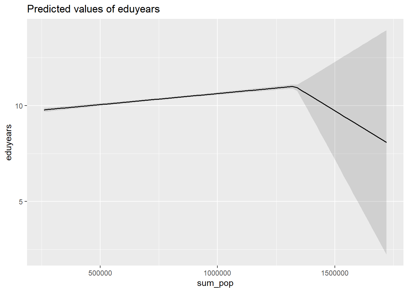

Figure 19: The significance of the population in the region on the level of education, Year 1985 - 2018

plot_model (mmodel, type = "pred", terms = c("sum_pop"))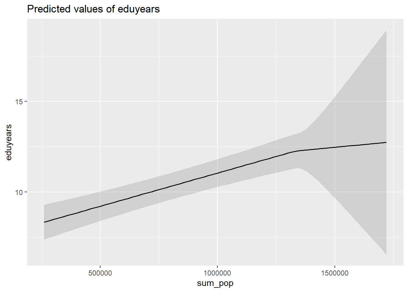

Figure 20: The significance of the population in the region on the level of education, Year 1985 - 2018

plot_model (pmodel, type = "pred", terms = c("sum_pop"))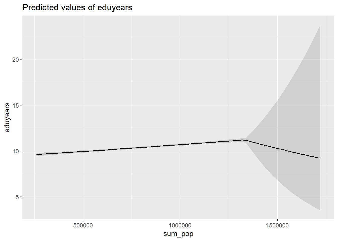

Figure 21: The significance of the population in the region on the level of education, Year 1985 - 2018

plot_model (model, type = "pred", terms = c("sum_edu_region_year"))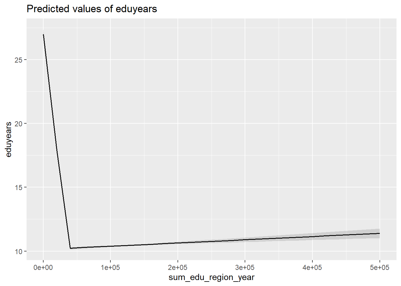

Figure 22: The significance of the number of persons with the same level of education, region and year on the level of education, Year 1985 - 2018

plot_model (mmodel, type = "pred", terms = c("sum_edu_region_year"))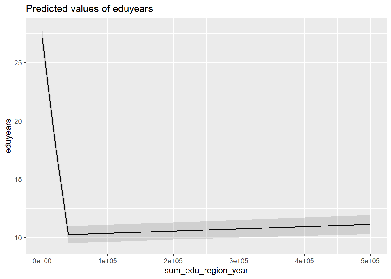

Figure 23: The significance of the number of persons with the same level of education, region and year on the level of education, Year 1985 - 2018

plot_model (pmodel, type = "pred", terms = c("sum_edu_region_year"))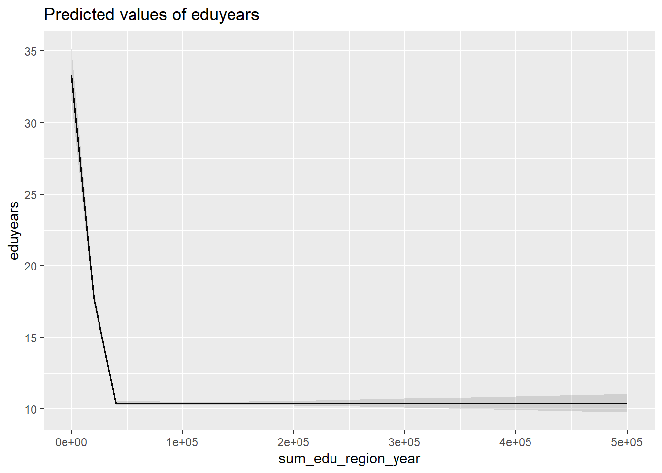

Figure 24: The significance of the number of persons with the same level of education, region and year on the level of education, Year 1985 - 2018

tbnum %>%
  ggplot () +  
    geom_point (mapping = aes(x = sum_edu_region_year, y = eduyears)) + 
  labs(
    x = "# persons with same edulevel, region, year",
    y = "Years of education"
  )

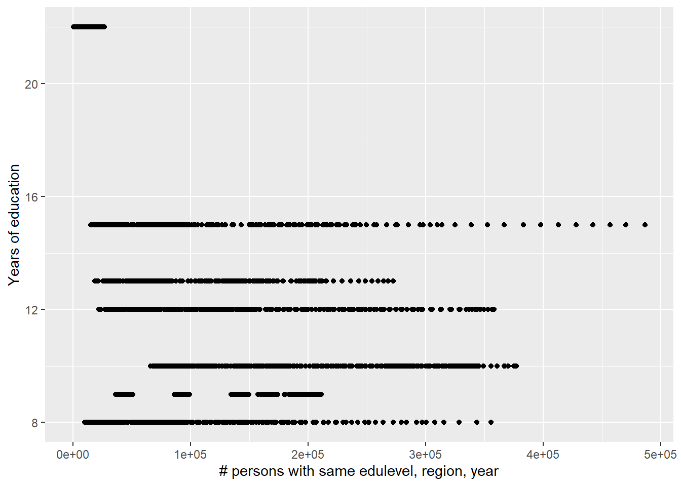
Figure 25: The significance of the number of persons with the same level of education, region and year on the level of education, Year 1985 - 2018

plot_model (model, type = "pred", terms = c("perc_women", "sum_pop"))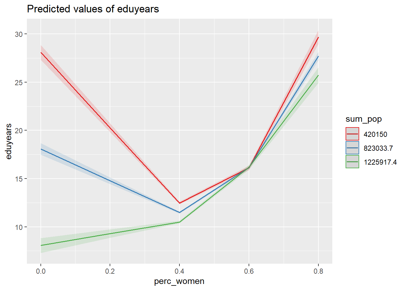

Figure 26: The significance of the interaction between per cent women and population in the region on the level of education, Year 1985 - 2018

plot_model (mmodel, type = "pred", terms = c("perc_women", "sum_pop"))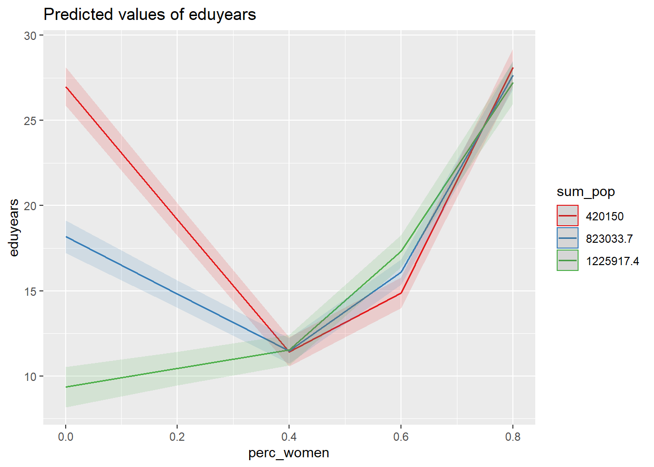

Figure 27: The significance of the interaction between per cent women and population in the region on the level of education, Year 1985 - 2018

plot_model (pmodel, type = "pred", terms = c("perc_women", "sum_pop"))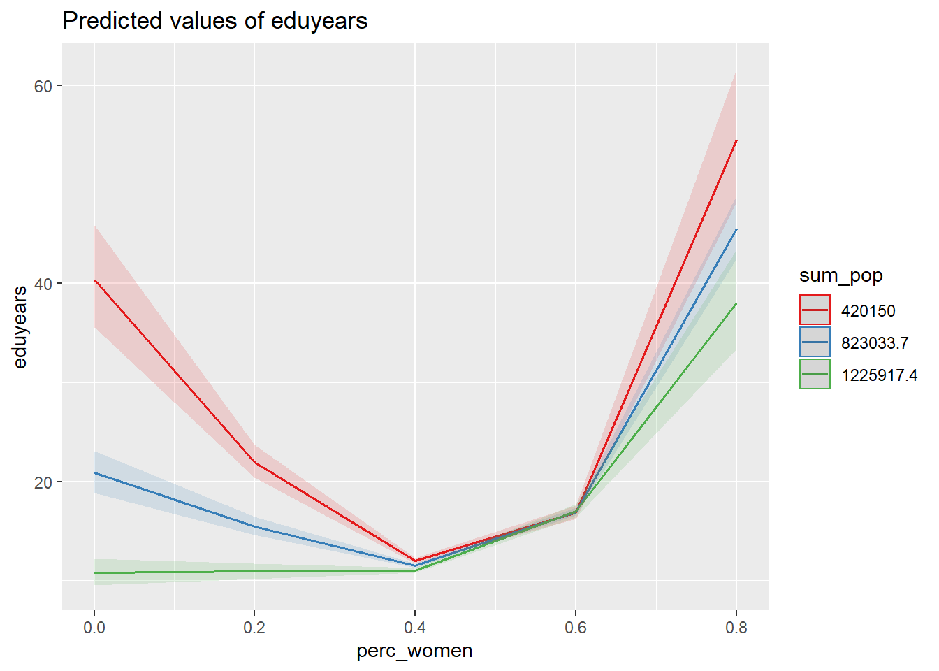

Figure 28: The significance of the interaction between per cent women and population in the region on the level of education, Year 1985 - 2018

tbnum %>%
  ggplot () +  
    geom_jitter (mapping = aes(x = perc_women, y = eduyears, colour = sum_pop)) + 
  labs(
    x = "Percent women",
    y = "Years of education"
  )

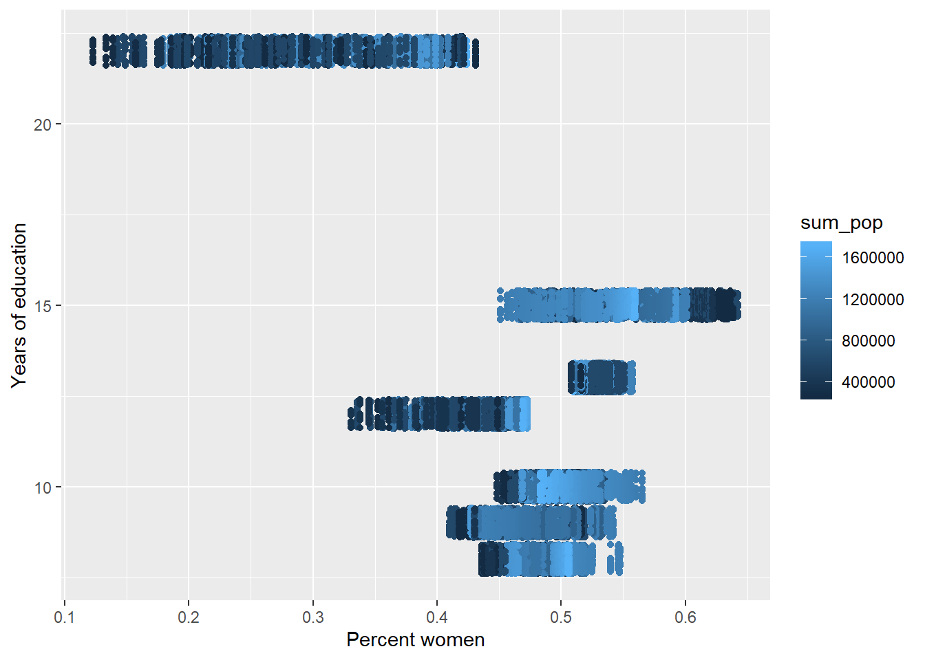
Figure 29: The significance of the interaction between per cent women and population in the region on the level of education, Year 1985 - 2018

plot_model (model, type = "pred", terms = c("year_n", "sum_pop"))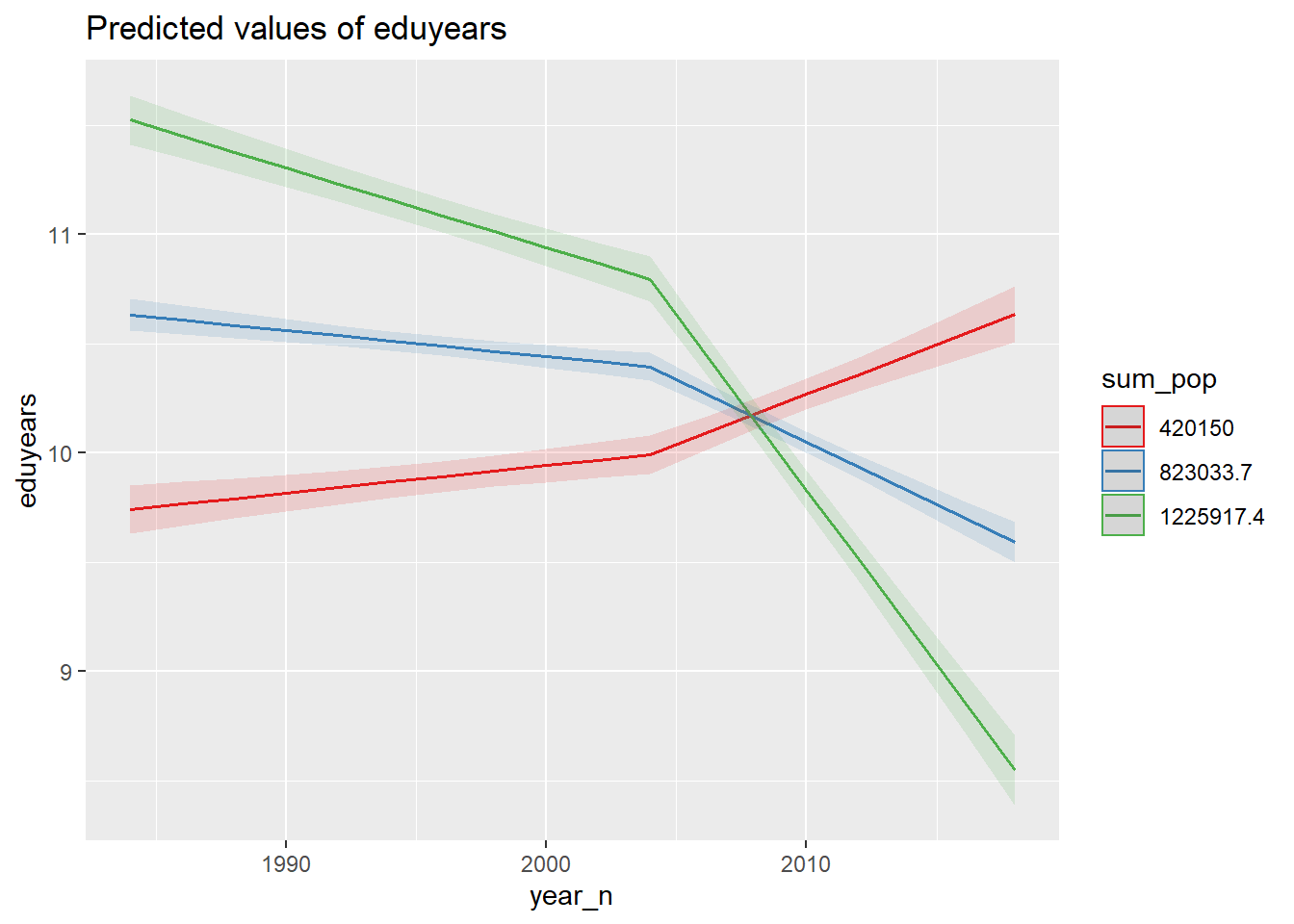

Figure 30: The significance of the interaction between the population in the region and year on the level of education, Year 1985 - 2018

plot_model (mmodel, type = "pred", terms = c("year_n", "sum_pop"))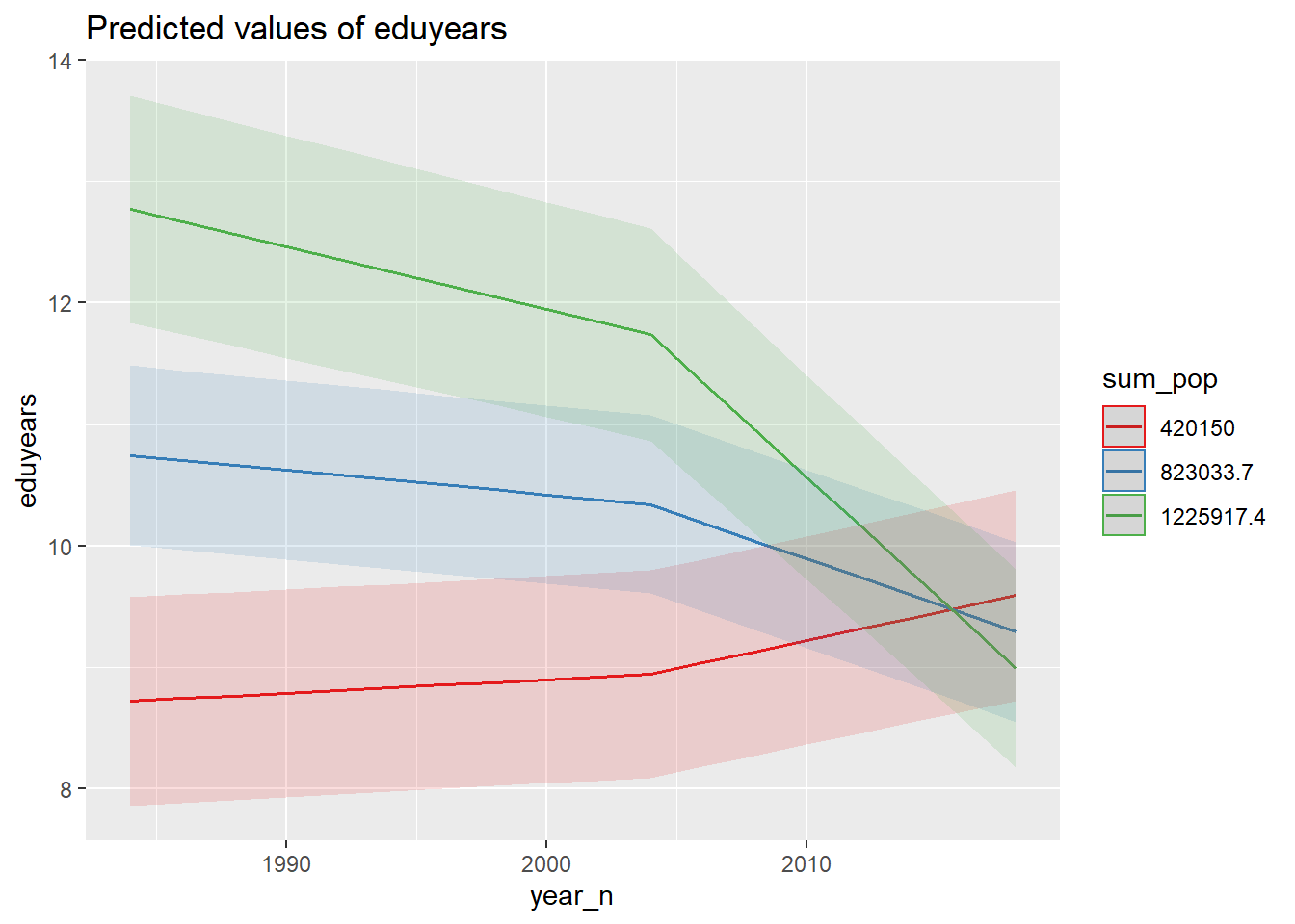

Figure 31: The significance of the interaction between the population in the region and year on the level of education, Year 1985 - 2018

plot_model (pmodel, type = "pred", terms = c("year_n", "sum_pop"))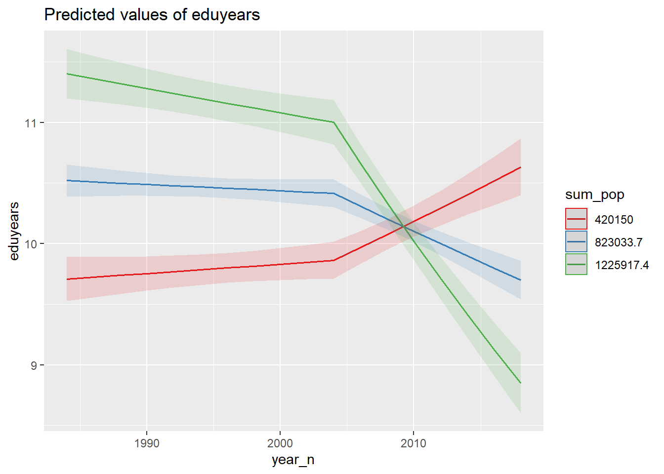

Figure 32: The significance of the interaction between the population in the region and year on the level of education, Year 1985 - 2018

tbnum %>%
  ggplot () +  
    geom_jitter (mapping = aes(x = sum_pop, y = eduyears, colour = year_n)) + 
  labs(
    x = "Population in region",
    y = "Years of education"
  )

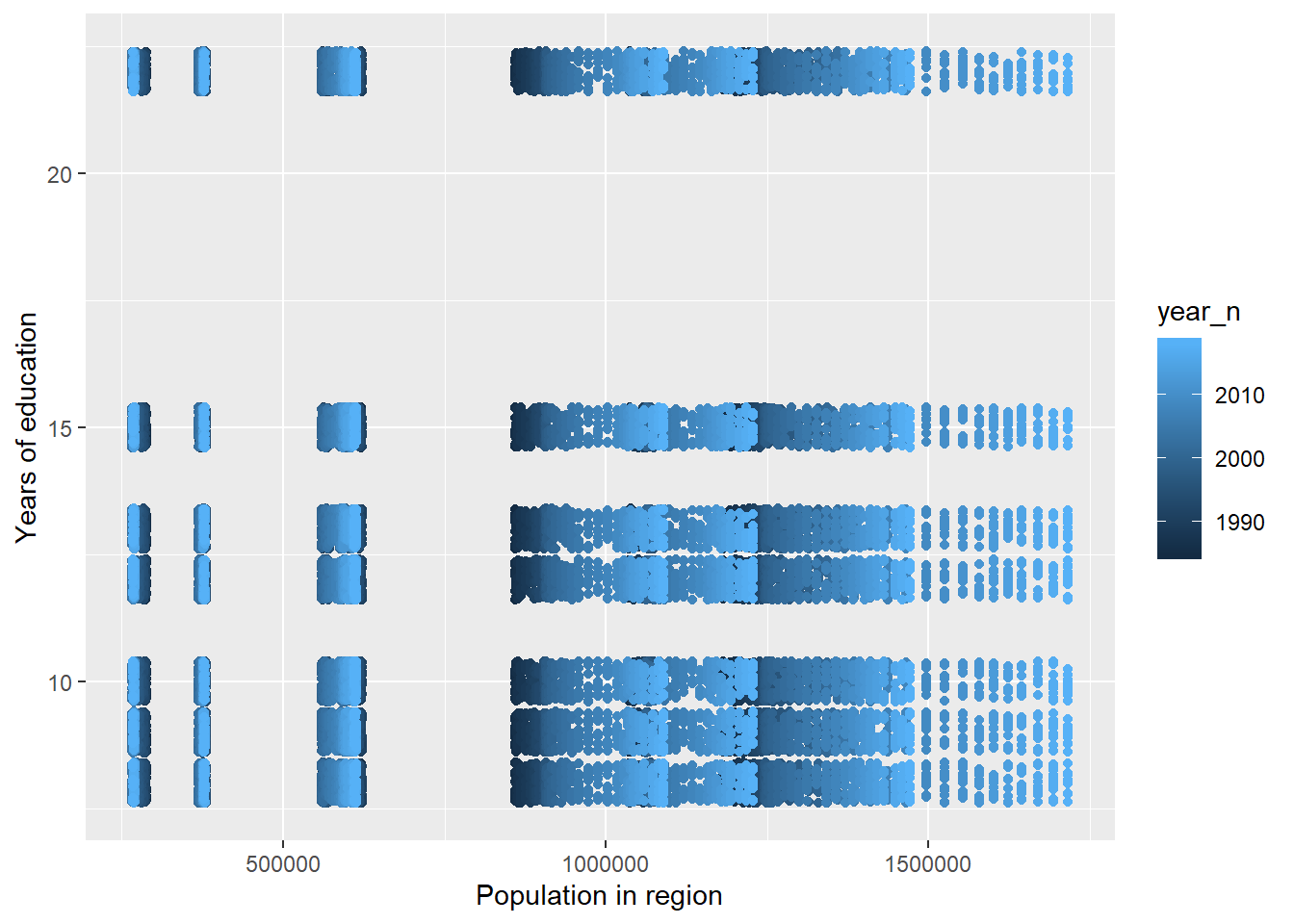
Figure 33: The significance of the interaction between the population in the region and year on the level of education, Year 1985 - 2018

plot_model (model, type = "pred", terms = c("sum_edu_region_year", "sum_pop"))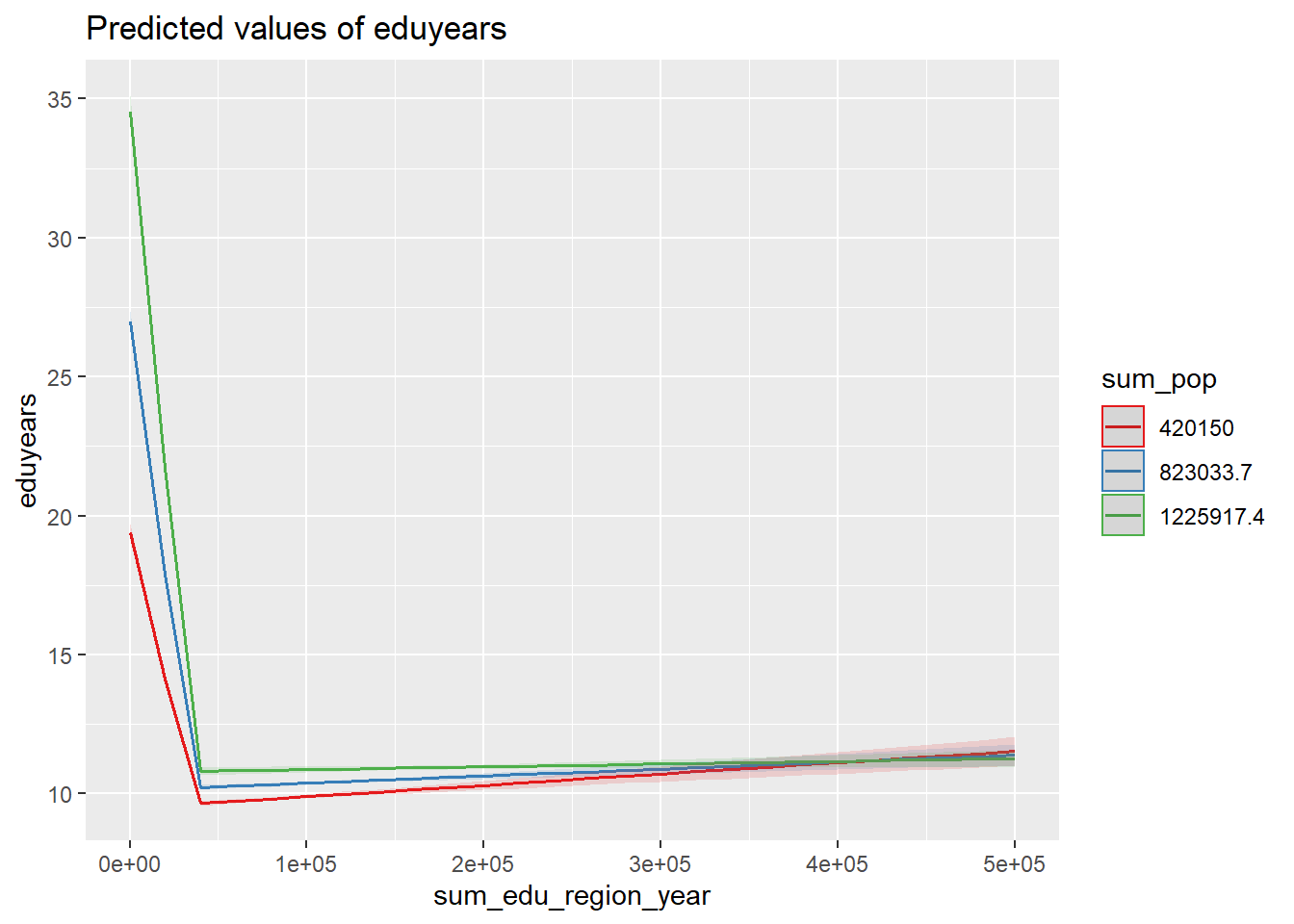

The significance of the interaction between the number of persons with the same level of education, region and year and population in the region on the level of education, Year 1985 - 2018

Figure 34: The significance of the interaction between the number of persons with the same level of education, region and year and population in the region on the level of education, Year 1985 - 2018

plot_model (mmodel, type = "pred", terms = c("sum_edu_region_year", "sum_pop"))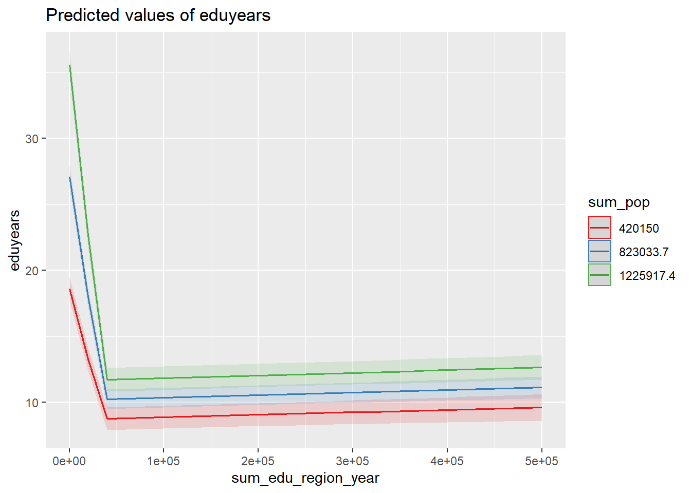

Figure 35: The significance of the interaction between the number of persons with the same level of education, region and year and population in the region on the level of education, Year 1985 - 2018

plot_model (pmodel, type = "pred", terms = c("sum_edu_region_year", "sum_pop"))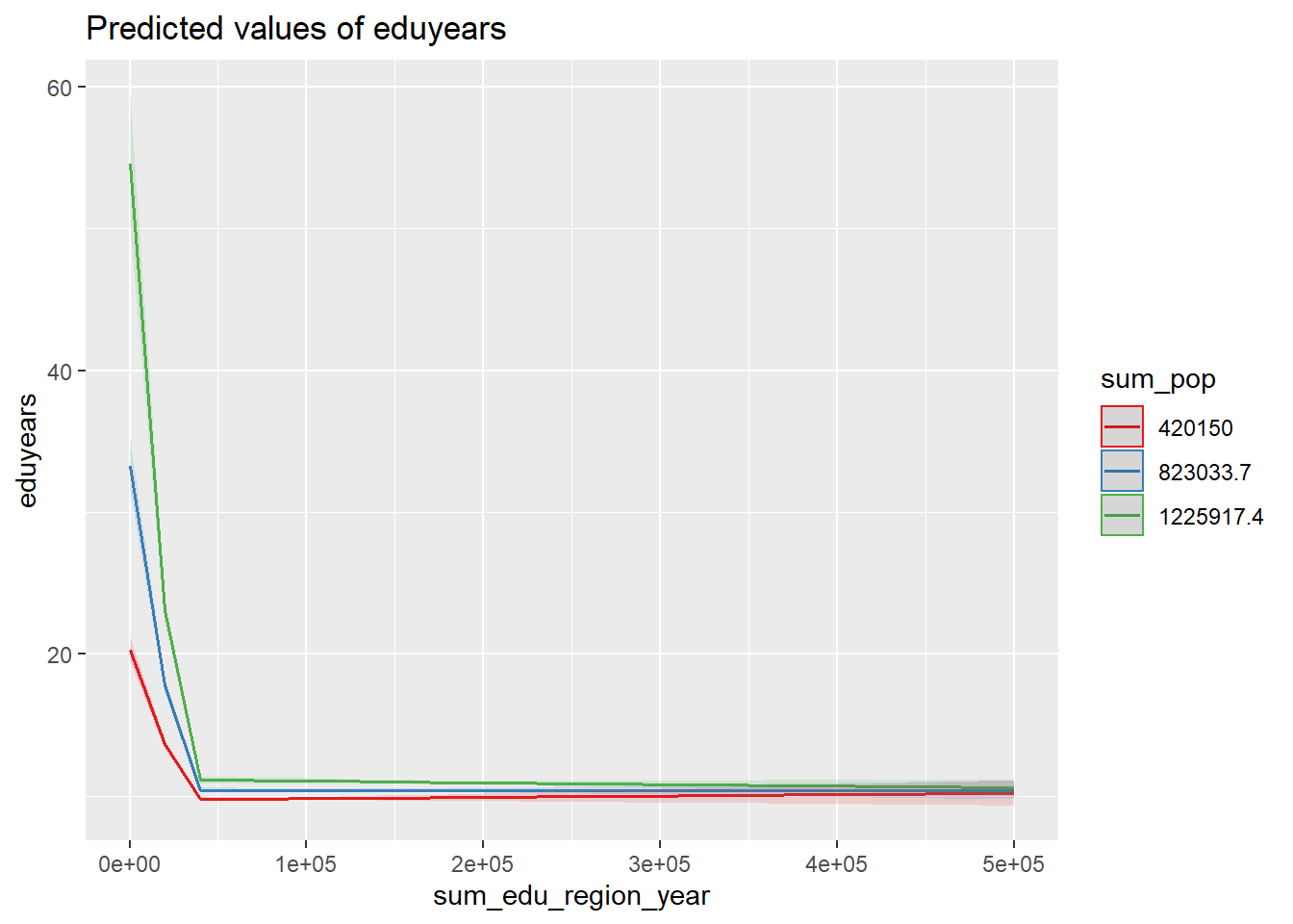

Figure 36: The significance of the interaction between the number of persons with the same level of education, region and year and population in the region on the level of education, Year 1985 - 2018

tbnum %>%
  ggplot () +  
    geom_jitter (mapping = aes(x = sum_edu_region_year, y = eduyears, colour = sum_pop)) + 
  labs(
    x = "# persons with same edulevel, region, year",
    y = "Years of education"
  )

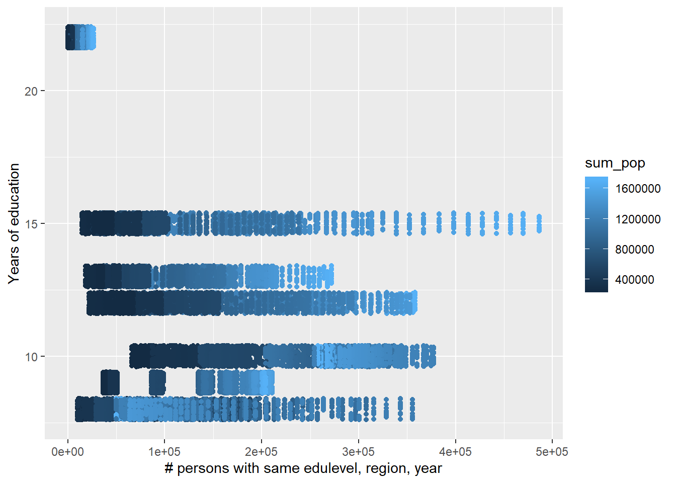
Figure 37: The significance of the interaction between the number of persons with the same level of education, region and year and population in the region on the level of education, Year 1985 - 2018

plot_model (model, type = "pred", terms = c("year_n", "perc_women"))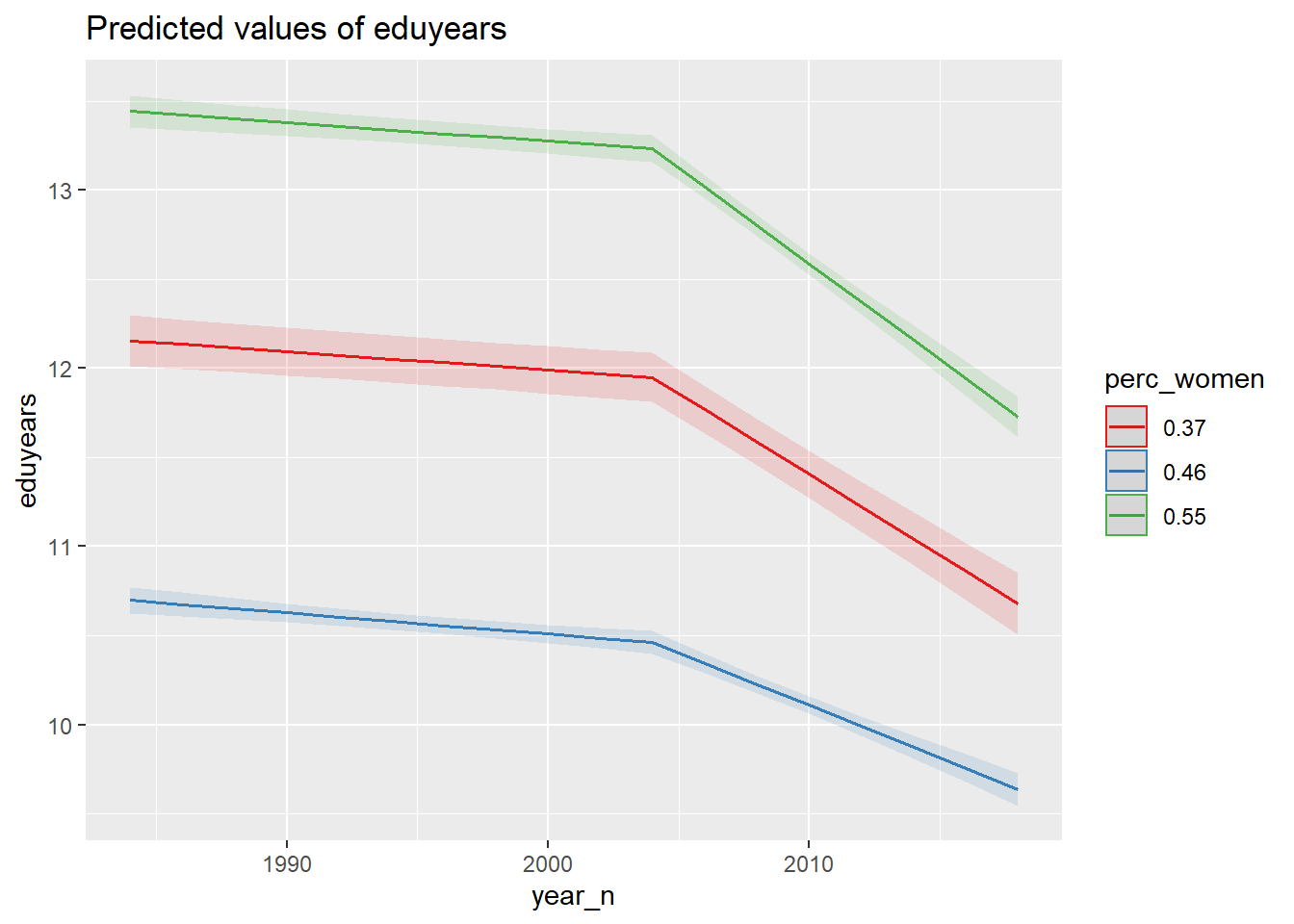

Figure 38: The significance of the interaction between per cent women and year on the level of education, Year 1985 - 2018

plot_model (mmodel, type = "pred", terms = c("year_n", "perc_women"))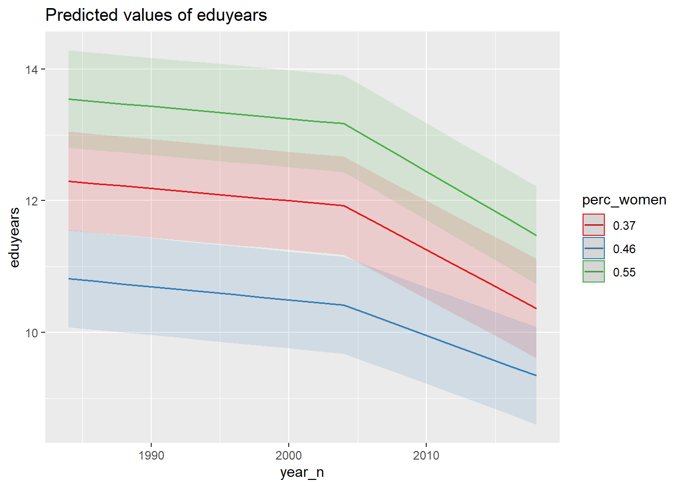

Figure 39: The significance of the interaction between per cent women and year on the level of education, Year 1985 - 2018

plot_model (pmodel, type = "pred", terms = c("year_n", "perc_women"))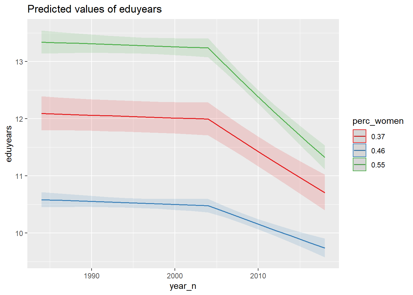

Figure 40: The significance of the interaction between per cent women and year on the level of education, Year 1985 - 2018

tbnum %>%
  ggplot () +  
    geom_jitter (mapping = aes(x = perc_women, y = eduyears, colour = year_n)) + 
  labs(
    x = "Percent women",
    y = "Years of education"
  )

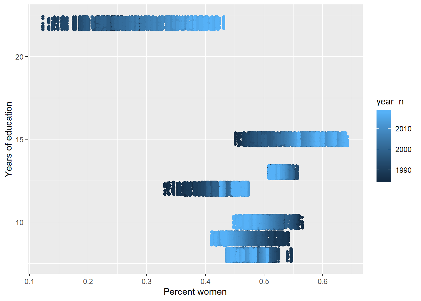
Figure 41: The significance of the interaction between per cent women and year on the level of education, Year 1985 - 2018

plot_model (model, type = "pred", terms = c("perc_women", "sum_edu_region_year"))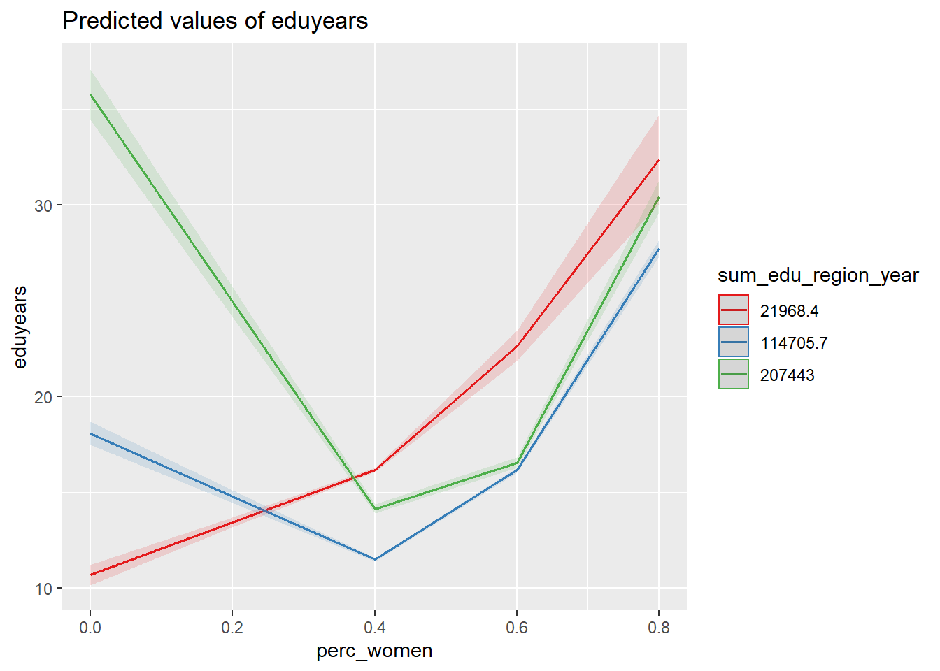

The significance of the interaction between the number of persons with the same level of education, region and year and per cent women on the level of education, Year 1985 - 2018

Figure 42: The significance of the interaction between the number of persons with the same level of education, region and year and per cent women on the level of education, Year 1985 - 2018

plot_model (mmodel, type = "pred", terms = c("perc_women", "sum_edu_region_year"))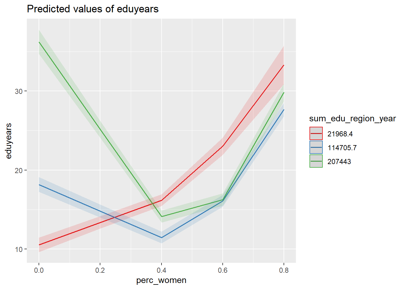

Figure 43: The significance of the interaction between the number of persons with the same level of education, region and year and per cent women on the level of education, Year 1985 - 2018

plot_model (pmodel, type = "pred", terms = c("perc_women", "sum_edu_region_year"))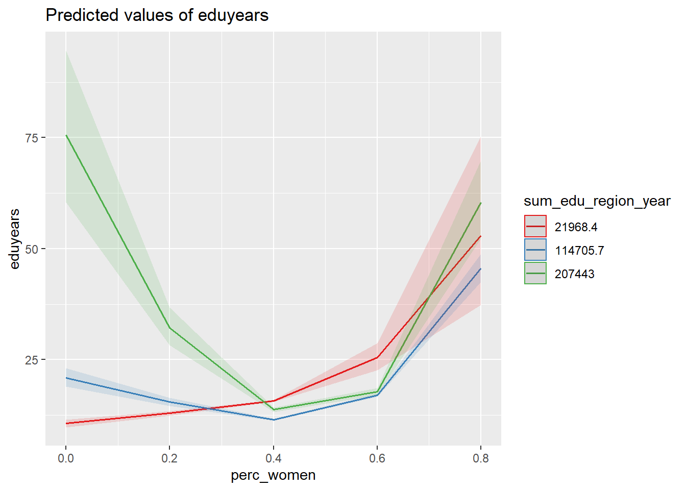

Figure 44: The significance of the interaction between the number of persons with the same level of education, region and year and per cent women on the level of education, Year 1985 - 2018

tbnum %>%
  ggplot () +  
    geom_jitter (mapping = aes(x = sum_edu_region_year, y = eduyears, colour = perc_women)) + 
  labs(
    x = "# persons with same edulevel, region, year",
    y = "Years of education"
  )

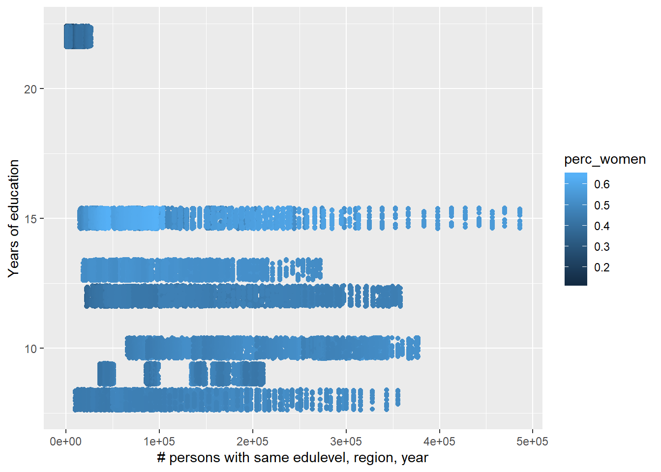
Figure 45: The significance of the interaction between the number of persons with the same level of education, region and year and per cent women on the level of education, Year 1985 - 2018

plot_model (model, type = "pred", terms = c("year_n", "sum_edu_region_year"))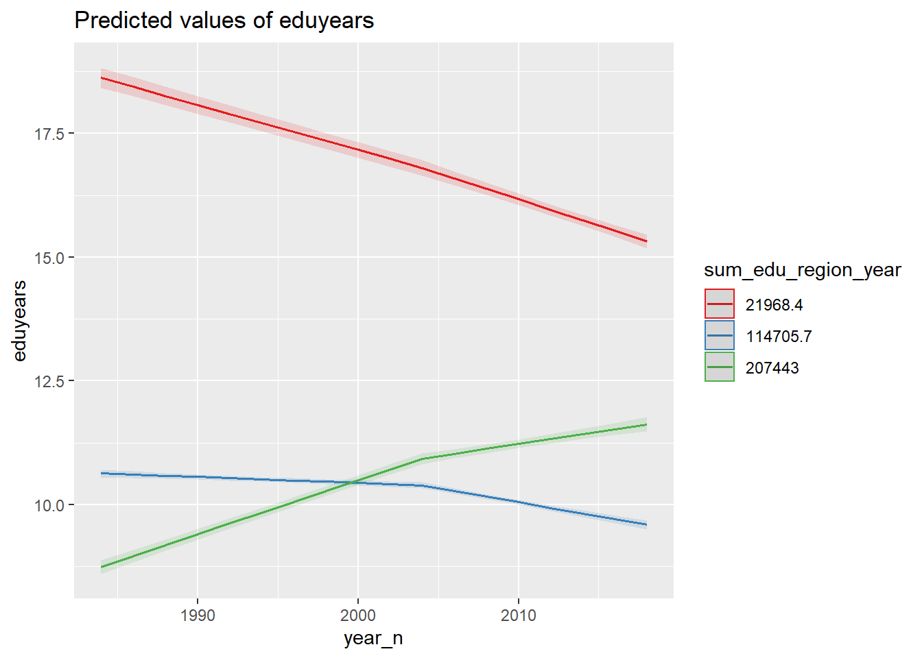

The significance of the interaction between year and the number of persons with the same level of education, region and year on the level of education, Year 1985 - 2018

Figure 46: The significance of the interaction between year and the number of persons with the same level of education, region and year on the level of education, Year 1985 - 2018

plot_model (mmodel, type = "pred", terms = c("year_n", "sum_edu_region_year"))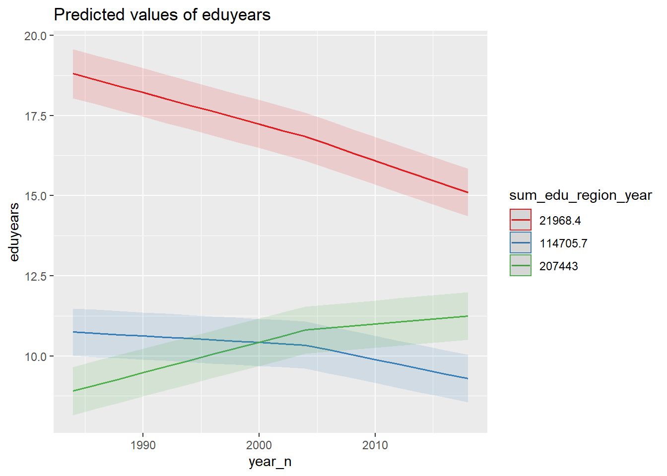

Figure 47: The significance of the interaction between year and the number of persons with the same level of education, region and year on the level of education, Year 1985 - 2018

plot_model (pmodel, type = "pred", terms = c("year_n", "sum_edu_region_year"))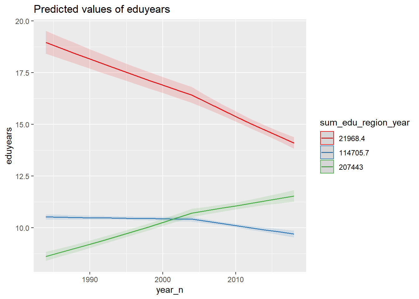

Figure 48: The significance of the interaction between year and the number of persons with the same level of education, region and year on the level of education, Year 1985 - 2018

tbnum %>%
  ggplot () +  
    geom_jitter (mapping = aes(x = sum_edu_region_year, y = eduyears, colour = year_n)) + 
  labs(
    x = "# persons with same edulevel, region, year",
    y = "Years of education"
  )

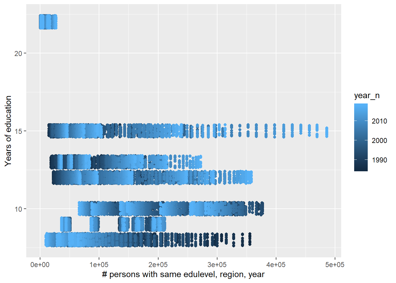
Figure 49: The significance of the interaction between year and the number of persons with the same level of education, region and year on the level of education, Year 1985 - 2018