In my last post, I analysed how the level of education is affected by region, sex and year. In this post, I will continue with the same dataset but this time I will include age in the analysis. Please send suggestions for improvement of the analysis to ranalystatisticssweden@gmail.com.
First, define libraries and functions.
library (tidyverse)## -- Attaching packages -------------------------------------------------- tidyverse 1.3.0 --## v ggplot2 3.2.1 v purrr 0.3.3
## v tibble 2.1.3 v dplyr 0.8.3
## v tidyr 1.0.2 v stringr 1.4.0
## v readr 1.3.1 v forcats 0.4.0## -- Conflicts ----------------------------------------------------- tidyverse_conflicts() --
## x dplyr::filter() masks stats::filter()
## x dplyr::lag() masks stats::lag()library (broom)
library (car)## Loading required package: carData##
## Attaching package: 'car'## The following object is masked from 'package:dplyr':
##
## recode## The following object is masked from 'package:purrr':
##
## somelibrary (sjPlot)## Registered S3 methods overwritten by 'lme4':
## method from
## cooks.distance.influence.merMod car
## influence.merMod car
## dfbeta.influence.merMod car
## dfbetas.influence.merMod carlibrary (leaps)
library (MASS)##
## Attaching package: 'MASS'## The following object is masked from 'package:dplyr':
##
## selectlibrary (earth)## Warning: package 'earth' was built under R version 3.6.3## Loading required package: Formula## Loading required package: plotmo## Warning: package 'plotmo' was built under R version 3.6.3## Loading required package: plotrix## Loading required package: TeachingDemos## Warning: package 'TeachingDemos' was built under R version 3.6.3library (acepack)## Warning: package 'acepack' was built under R version 3.6.3library (lspline)## Warning: package 'lspline' was built under R version 3.6.3library (lme4)## Loading required package: Matrix##
## Attaching package: 'Matrix'## The following objects are masked from 'package:tidyr':
##
## expand, pack, unpacklibrary (pROC)## Warning: package 'pROC' was built under R version 3.6.3## Type 'citation("pROC")' for a citation.##
## Attaching package: 'pROC'## The following objects are masked from 'package:stats':
##
## cov, smooth, varlibrary (boot)##
## Attaching package: 'boot'## The following object is masked from 'package:car':
##
## logitlibrary (faraway)##
## Attaching package: 'faraway'## The following objects are masked from 'package:boot':
##
## logit, melanoma## The following objects are masked from 'package:car':
##
## logit, viflibrary (arm)## Warning: package 'arm' was built under R version 3.6.3##
## arm (Version 1.10-1, built: 2018-4-12)## Working directory is C:/R/rblog/content/post##
## Attaching package: 'arm'## The following objects are masked from 'package:faraway':
##
## fround, logit, pfround## The following object is masked from 'package:boot':
##
## logit## The following object is masked from 'package:plotrix':
##
## rescale## The following object is masked from 'package:car':
##
## logitreadfile <- function (file1){read_csv (file1, col_types = cols(), locale = readr::locale (encoding = "latin1"), na = c("..", "NA")) %>%
gather (starts_with("19"), starts_with("20"), key = "year", value = groupsize) %>%
drop_na() %>%
mutate (year_n = parse_number (year))
}
perc_women <- function(x){
ifelse (length(x) == 2, x[2] / (x[1] + x[2]), NA)
}
nuts <- read.csv("nuts.csv") %>%
mutate(NUTS2_sh = substr(NUTS2, 3, 4))The data table is downloaded from Statistics Sweden. It is saved as a comma-delimited file without heading, UF0506A1.csv, http://www.statistikdatabasen.scb.se/pxweb/en/ssd/.
I will calculate the percentage of women in for the different education levels in the different regions for each year. In my later analysis, I will use the number of people in each education level, region, year and age.
The table: Population 16-74 years of age by region, highest level of education, age and sex. Year 1985 - 2018 NUTS 2 level 2008- 10 year intervals (16-74)
The data is aggregated, the size of each group is in the column groupsize.
tb <- readfile("UF0506A1.csv") %>%
  mutate(edulevel = `level of education`) %>%
  group_by(edulevel, region, year, sex, age) %>%
  mutate(groupsize_age = sum(groupsize)) %>%
  group_by(edulevel, region, year, age) %>%
  mutate (sum_edu_region_year = sum(groupsize)) %>%
  mutate (perc_women = perc_women (groupsize_age)) %>%
  group_by(region, year) %>%
  mutate (sum_pop = sum(groupsize)) %>% rowwise() %>%
  mutate(age_l = unlist(lapply(strsplit(substr(age, 1, 5), "-"), strtoi))[1]) %>%
  rowwise() %>%
  mutate(age_h = unlist(lapply(strsplit(substr(age, 1, 5), "-"), strtoi))[2]) %>%
  mutate(age_n = (age_l + age_h) / 2) %>%
  left_join(nuts %>% distinct (NUTS2_en, NUTS2_sh), by = c("region" = "NUTS2_en"))
## Warning: Column `region`/`NUTS2_en` joining character vector and factor,
## coercing into character vectornumedulevel <- read.csv("edulevel_1.csv")
numedulevel[, 2] <- data.frame(c(8, 9, 10, 12, 13, 15, 22, NA))
numedulevel %>%
knitr::kable(
booktabs = TRUE,
caption = 'Calculated in previous post, length of education') | level.of.education | eduyears |
|---|---|
| primary and secondary education less than 9 years (ISCED97 1) | 8 |
| primary and secondary education 9-10 years (ISCED97 2) | 9 |
| upper secondary education, 2 years or less (ISCED97 3C) | 10 |
| upper secondary education 3 years (ISCED97 3A) | 12 |
| post-secondary education, less than 3 years (ISCED97 4+5B) | 13 |
| post-secondary education 3 years or more (ISCED97 5A) | 15 |
| post-graduate education (ISCED97 6) | 22 |
| no information about level of educational attainment | NA |
tbnum <- tb %>%
  right_join(numedulevel, by = c("level of education" = "level.of.education")) %>%
  filter(!is.na(eduyears)) %>%
  drop_na()
## Warning: Column `level of education`/`level.of.education` joining character
## vector and factor, coercing into character vectortbnum %>%
filter (year_n == 2018) %>%
ggplot () +
geom_point (mapping = aes(x = NUTS2_sh,y = perc_women, colour = age_n)) +
facet_grid(. ~ eduyears)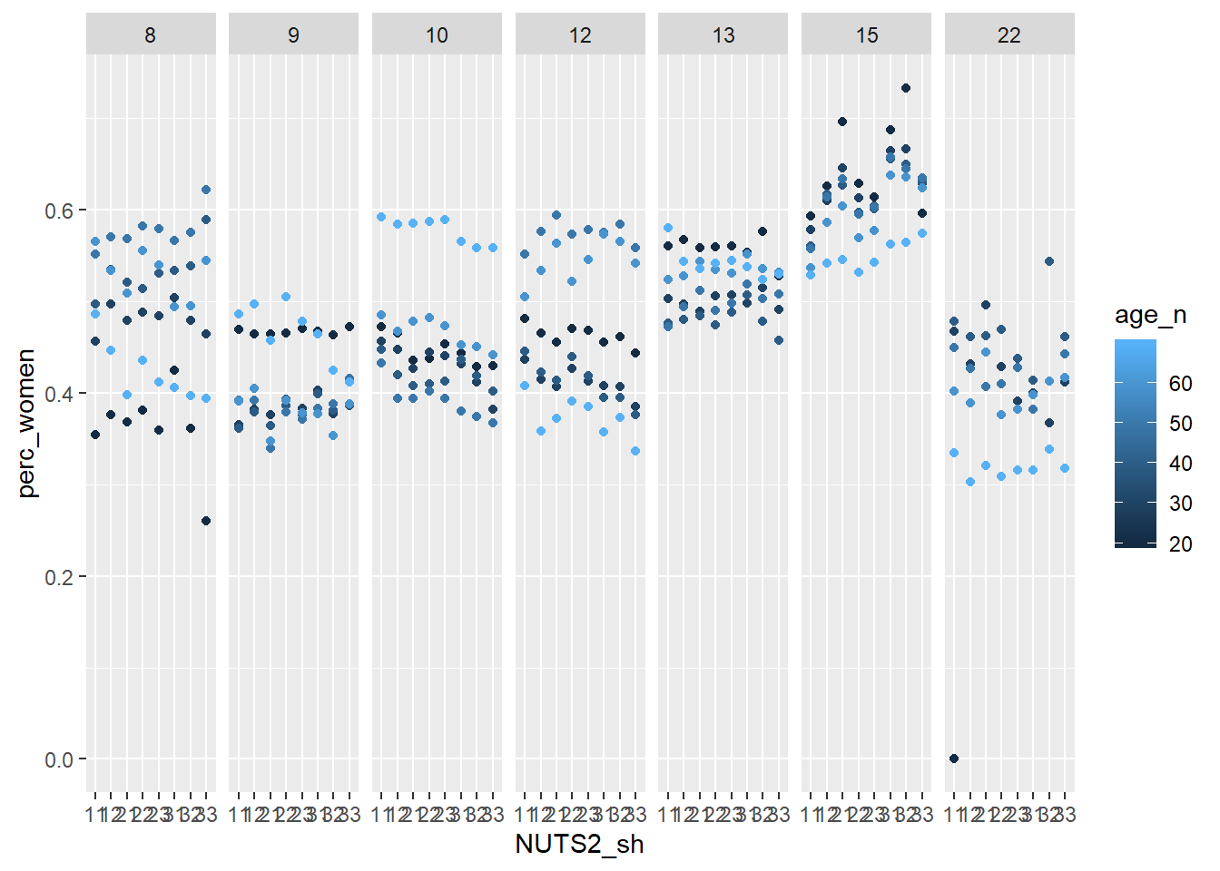
Figure 1: Population by region, level of education, percent women and year, Year 1985 - 2018
tbnum %>%
  filter (year_n == 2008) %>%
  ggplot () +
    geom_point (mapping = aes(x = NUTS2_sh,y = perc_women, colour = age_n)) +
  facet_grid(. ~ eduyears)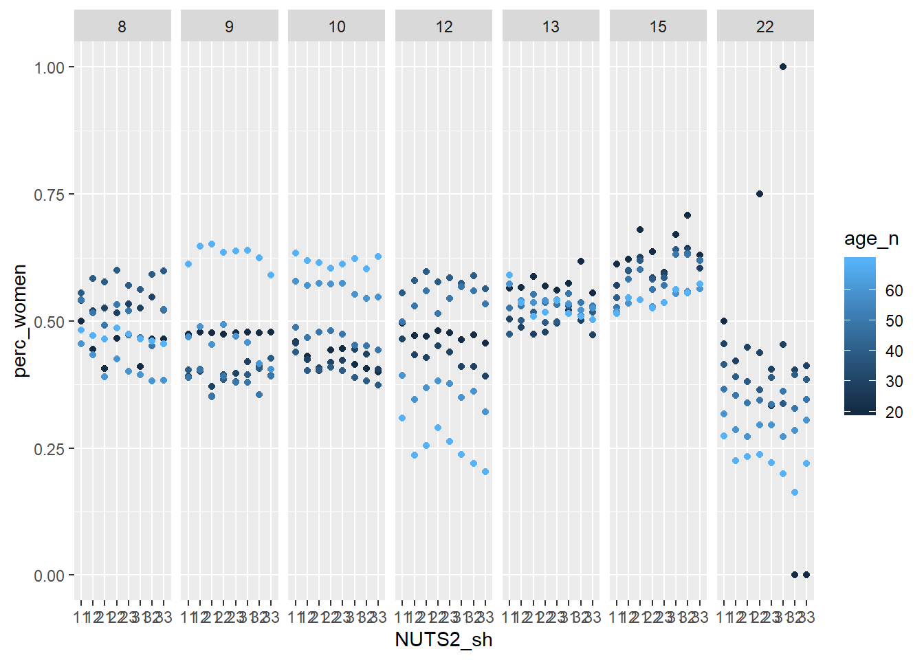
Figure 2: Population by region, level of education, percent women and year, Year 1985 - 2018
tbnum %>%
  filter (year_n == 1998) %>%
  ggplot () +
    geom_point (mapping = aes(x = NUTS2_sh,y = perc_women, colour = age_n)) +
  facet_grid(. ~ eduyears)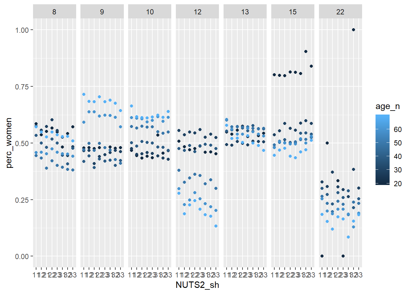
Figure 3: Population by region, level of education, percent women and year, Year 1985 - 2018
tbnum %>%
  filter (year_n == 1988) %>%
  ggplot () +
    geom_point (mapping = aes(x = NUTS2_sh,y = perc_women, colour = age_n)) +
  facet_grid(. ~ eduyears)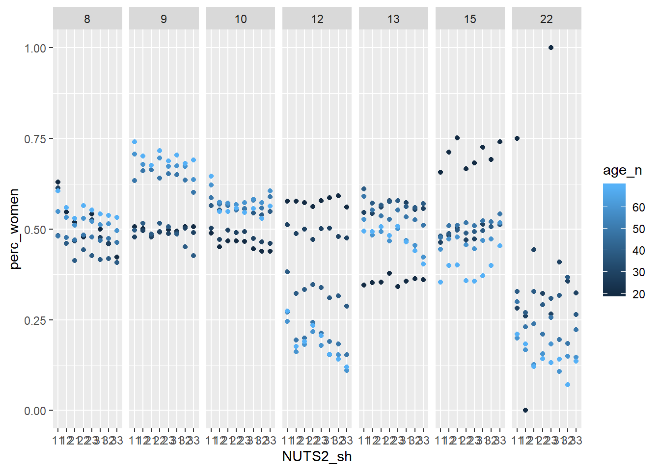
Figure 4: Population by region, level of education, percent women and year, Year 1985 - 2018
summary(tbnum)## region age level of education sex
## Length:22660 Length:22660 Length:22660 Length:22660
## Class :character Class :character Class :character Class :character
## Mode :character Mode :character Mode :character Mode :character
##
##
##
## year groupsize year_n edulevel
## Length:22660 Min. : 0 Min. :1985 Length:22660
## Class :character 1st Qu.: 1713 1st Qu.:1993 Class :character
## Mode :character Median : 5737 Median :2001 Mode :character
## Mean : 9638 Mean :2001
## 3rd Qu.:14135 3rd Qu.:2010
## Max. :77163 Max. :2018
## groupsize_age sum_edu_region_year perc_women sum_pop
## Min. : 0 Min. : 1 Min. :0.0000 Min. : 266057
## 1st Qu.: 1713 1st Qu.: 3566 1st Qu.:0.4090 1st Qu.: 560119
## Median : 5737 Median : 11566 Median :0.4875 Median : 859794
## Mean : 9638 Mean : 19276 Mean :0.4707 Mean : 824996
## 3rd Qu.:14135 3rd Qu.: 28287 3rd Qu.:0.5542 3rd Qu.:1200038
## Max. :77163 Max. :134645 Max. :1.0000 Max. :1716160
## age_l age_h age_n NUTS2_sh
## Min. :16.00 Min. :24.00 Min. :20.00 Length:22660
## 1st Qu.:25.00 1st Qu.:34.00 1st Qu.:29.50 Class :character
## Median :45.00 Median :54.00 Median :49.50 Mode :character
## Mean :40.37 Mean :49.21 Mean :44.79
## 3rd Qu.:55.00 3rd Qu.:64.00 3rd Qu.:59.50
## Max. :65.00 Max. :74.00 Max. :69.50
## eduyears
## Min. : 8.00
## 1st Qu.: 9.00
## Median :12.00
## Mean :12.64
## 3rd Qu.:15.00
## Max. :22.00Let’s investigate the shape of the function for the response and predictors. The shape of the predictors has a great impact on the rest of the analysis. I use acepack to fit a model and plot both the response and the predictors.
tbtest <- tbnum %>% dplyr::select(sum_pop, sum_edu_region_year, year_n, perc_women, age_n)

tbtest <- data.frame(tbtest)

acefit <- ace(tbtest, tbnum$eduyears, wt=tbtest$sum_edu_region_year)

plot(tbnum$eduyears, acefit$ty, xlab = "Years of education", ylab = "transformed years of education")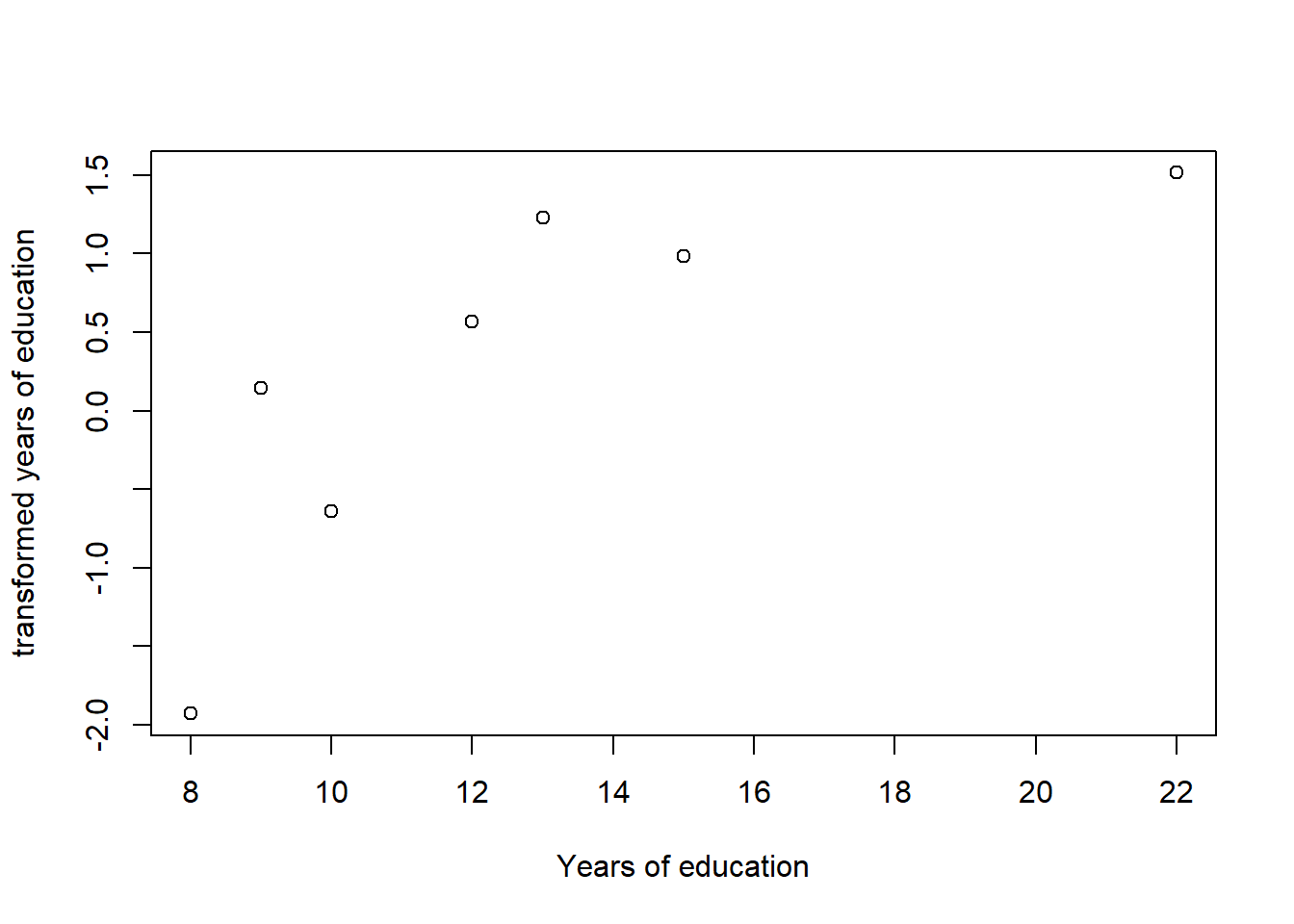
Figure 5: Plots of the response and predictors using acepack
plot(tbtest[,1], acefit$tx[,1], xlab = "Population in region", ylab = "transformed population in region")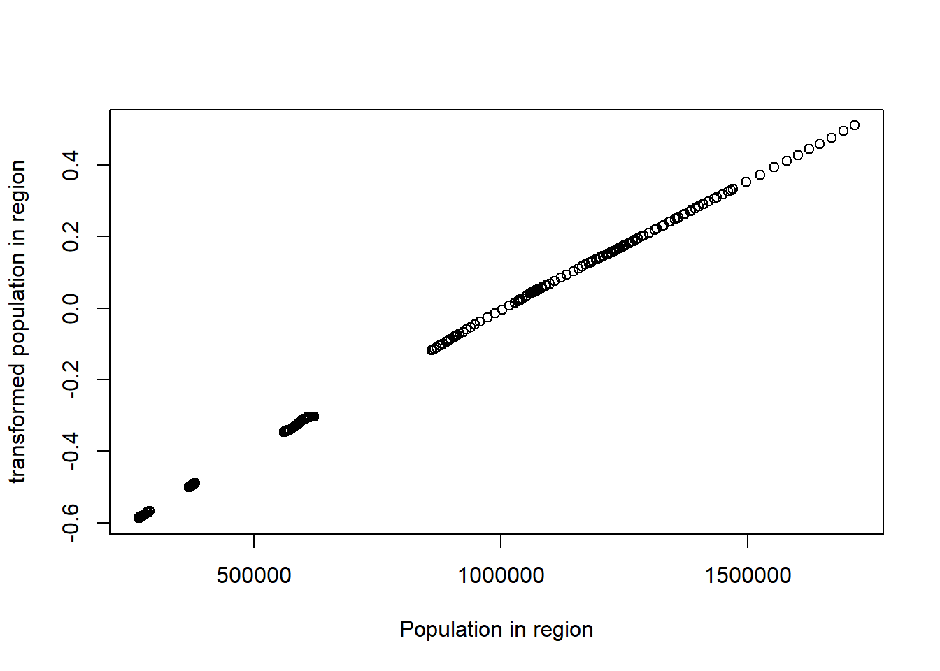
Figure 6: Plots of the response and predictors using acepack
plot(tbtest[,2], acefit$tx[,2], xlab = "# persons with same edulevel, region, year", ylab = "transformed # persons with same edulevel, region, year")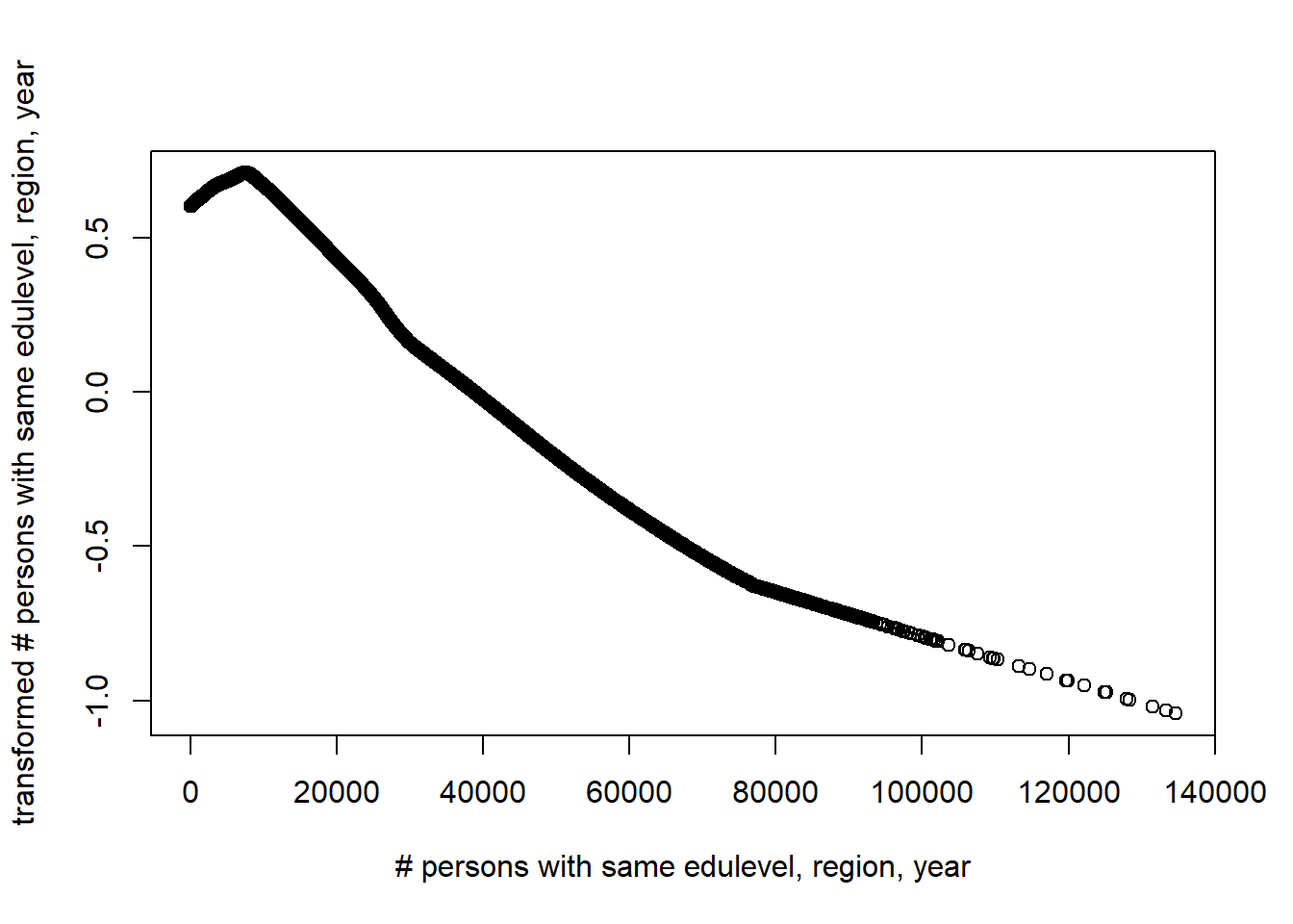
Figure 7: Plots of the response and predictors using acepack
plot(tbtest[,3], acefit$tx[,3], xlab = "Year", ylab = "transformed year")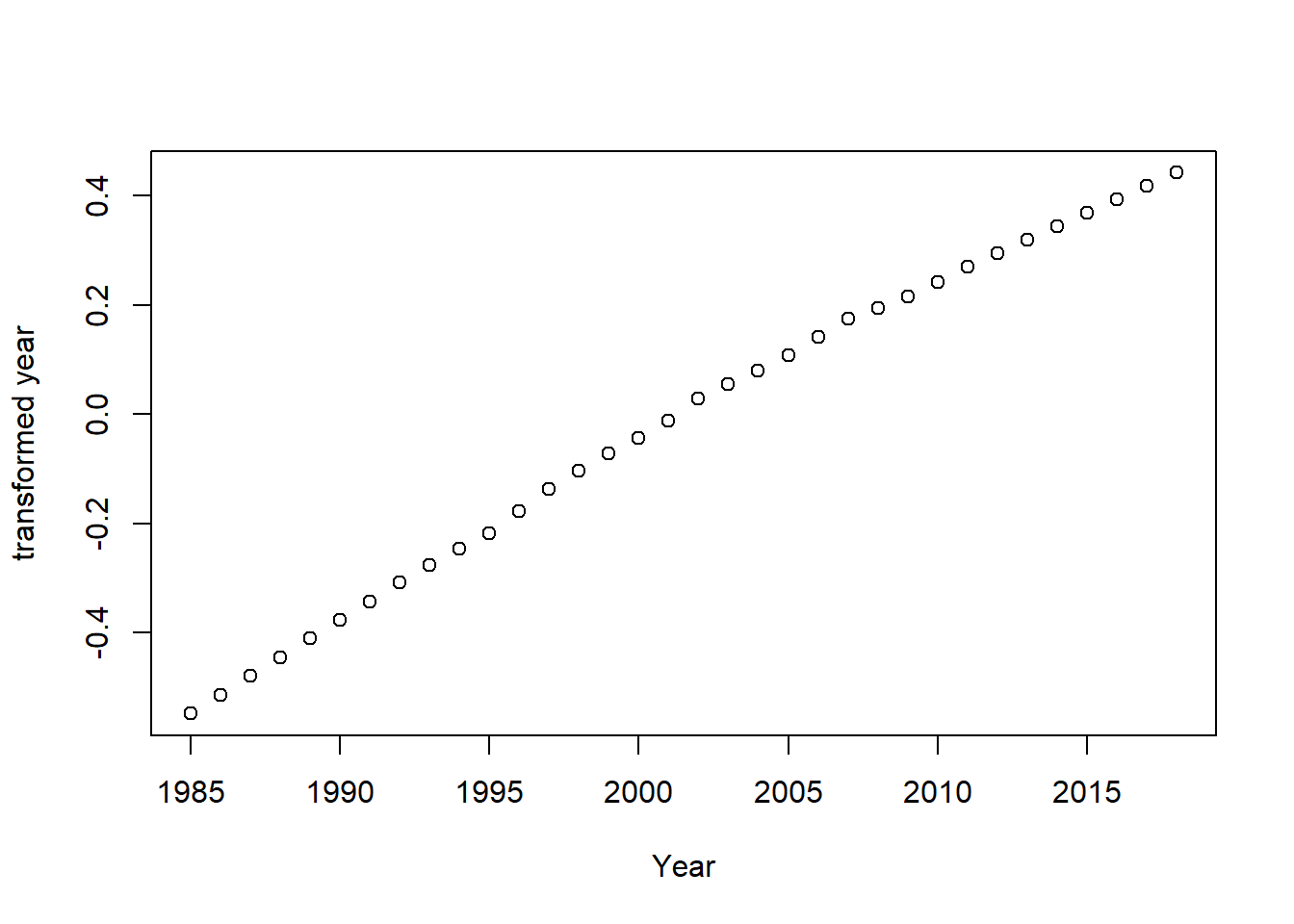
Figure 8: Plots of the response and predictors using acepack
plot(tbtest[,4], acefit$tx[,4], xlab = "Percent women", ylab = "transformed percent women")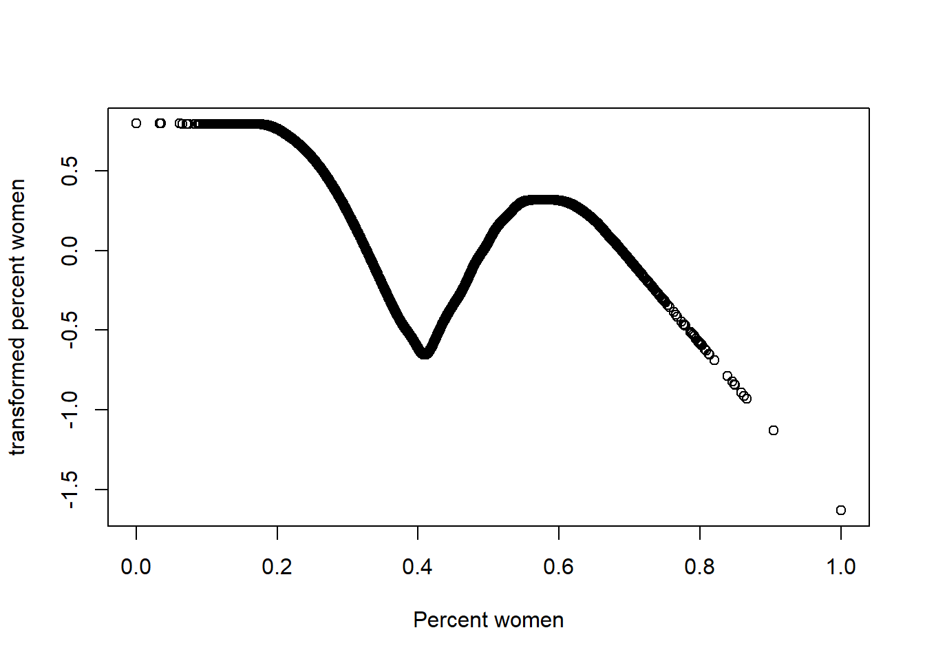
Figure 9: Plots of the response and predictors using acepack
plot(tbtest[,5], acefit$tx[,5], xlab = "Age", ylab = "transformed age")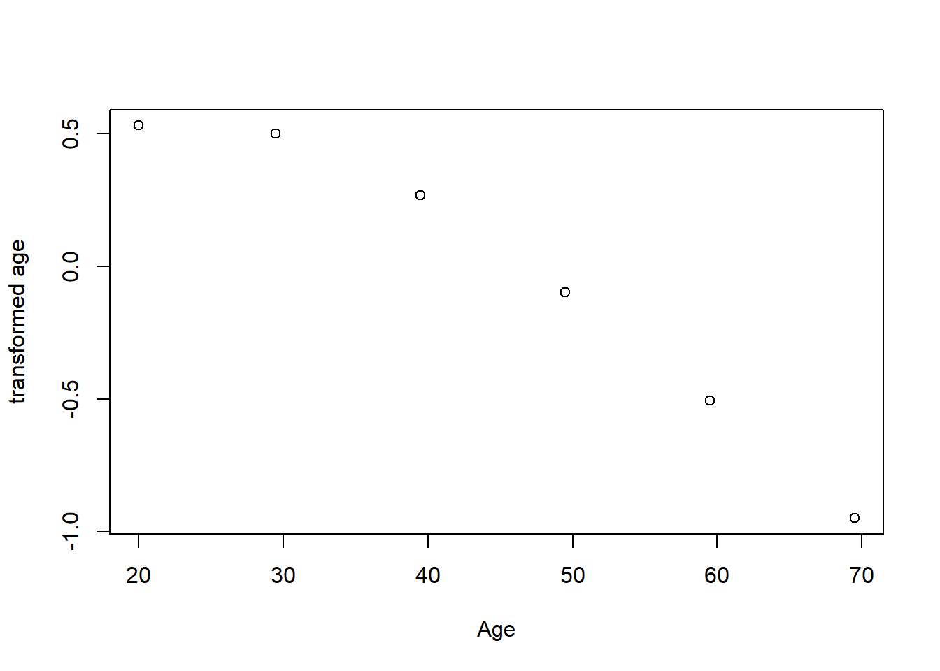
Figure 10: Plots of the response and predictors using acepack
I use MARS to fit hockey-stick functions for the predictors. I do not wish to overfit by using a better approximation at this point. I will include interactions of degree two. I will put more emphasis on groups with larger size by using the number of persons with same edulevel, region, year, age as weights in the regression. From the analysis with acepack, I will approximate the shape of the response with X^-1.
tbtemp <- tbnum %>% dplyr::select(eduyears, sum_pop, sum_edu_region_year, year_n, perc_women, age_n)

mmod <- earth(eduyears^-1 ~ ., weights = tbtest$sum_edu_region_year, data = tbtemp, nk = 9, degree = 2)

summary (mmod)
## Call: earth(formula=eduyears^-1~., data=tbtemp,
## weights=tbtest$sum_edu_region_year, degree=2, nk=9)
##
## coefficients
## (Intercept) 0.109974110
## h(68923-sum_edu_region_year) -0.000000172
## h(sum_edu_region_year-68923) -0.000000071
## h(0.402156-perc_women) -0.142039538
## h(perc_women-0.402156) -0.216582584
## h(2004-year_n) * h(perc_women-0.402156) 0.006151369
## h(year_n-2004) * h(perc_women-0.402156) -0.003086559
## h(perc_women-0.402156) * h(age_n-29.5) 0.004789032
## h(perc_women-0.402156) * h(29.5-age_n) 0.007923485
##
## Selected 9 of 9 terms, and 4 of 5 predictors
## Termination condition: Reached nk 9
## Importance: perc_women, age_n, year_n, sum_edu_region_year, sum_pop-unused
## Weights: 160, 160, 2503, 2503, 27984, 27984, 41596, 41596, 57813, 57813,...
## Number of terms at each degree of interaction: 1 4 4
## GCV 4.263981 RSS 96442.81 GRSq 0.3866042 RSq 0.3876866plot (mmod)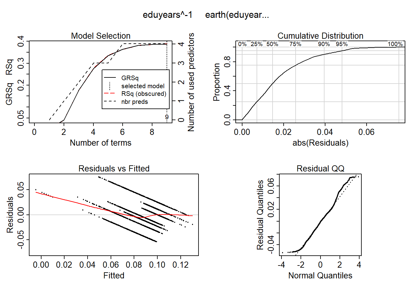
Figure 11: Hockey-stick functions fit with MARS for the predictors, Year 1985 - 2018
plotmo (mmod)## plotmo grid: sum_pop sum_edu_region_year year_n perc_women age_n
## 859794 11566.5 2001 0.4875054 49.5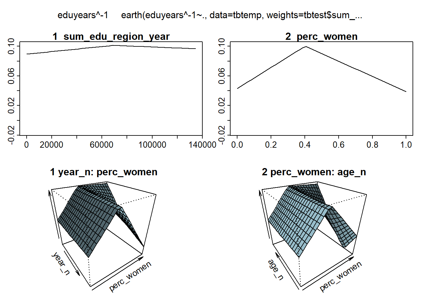
Figure 12: Hockey-stick functions fit with MARS for the predictors, Year 1985 - 2018
model_mmod <- lm (eduyears^-1 ~
  lspline(sum_edu_region_year, c(68923)) +
  lspline(perc_women, c(0.402156)) +
  lspline(year_n, c(2004)):lspline(perc_women, c(0.402156)) +
  lspline(perc_women, c(0.402156)):lspline(age_n, c(29.5)),
  weights = tbtest$sum_edu_region_year,
  data = tbnum)

summary (model_mmod)$r.squared
## [1] 0.4067181anova (model_mmod)## Analysis of Variance Table
##
## Response: eduyears^-1
## Df Sum Sq Mean Sq
## lspline(sum_edu_region_year, c(68923)) 2 6429 3214.4
## lspline(perc_women, c(0.402156)) 2 11182 5590.8
## lspline(perc_women, c(0.402156)):lspline(year_n, c(2004)) 4 18631 4657.7
## lspline(perc_women, c(0.402156)):lspline(age_n, c(29.5)) 4 27819 6954.8
## Residuals 22647 93445 4.1
## F value Pr(>F)
## lspline(sum_edu_region_year, c(68923)) 779.03 < 2.2e-16 ***
## lspline(perc_women, c(0.402156)) 1354.96 < 2.2e-16 ***
## lspline(perc_women, c(0.402156)):lspline(year_n, c(2004)) 1128.81 < 2.2e-16 ***
## lspline(perc_women, c(0.402156)):lspline(age_n, c(29.5)) 1685.54 < 2.2e-16 ***
## Residuals
## ---
## Signif. codes: 0 '***' 0.001 '**' 0.01 '*' 0.05 '.' 0.1 ' ' 1Since the predictors are on different scales I will also use MARS to fit hockey-stick functions to the standardised data. Weights can not be negative.
tbtemp <- tbnum %>% dplyr::select(eduyears, sum_pop, sum_edu_region_year, year_n, perc_women, age_n)

tbtemp_scale <- data.frame(tbtemp %>% scale())

mmod_scale <- earth(eduyears^-1 ~ ., weights = tbnum$sum_edu_region_year, data = tbtemp_scale, nk = 9, degree = 2)

summary (mmod_scale)
## Call: earth(formula=eduyears^-1~., data=tbtemp_scale,
## weights=tbnum$sum_edu_region_year, degree=2, nk=9)
##
## coefficients
## (Intercept) 1.4518768
## h(1.54673-sum_pop) -1.3123162
## h(2.48479-sum_edu_region_year) 2.2482786
## h(sum_edu_region_year-2.48479) 0.4668398
## h(0.589918-perc_women) -5.1021696
## h(perc_women-0.589918) -5.8909808
## h(-0.905736-age_n) -3.0330857
## h(age_n- -0.905736) -0.5385299
##
## Selected 8 of 9 terms, and 4 of 5 predictors
## Termination condition: Reached nk 9
## Importance: perc_women, sum_edu_region_year, sum_pop, age_n, year_n-unused
## Weights: 160, 160, 2503, 2503, 27984, 27984, 41596, 41596, 57813, 57813,...
## Number of terms at each degree of interaction: 1 7 (additive model)
## GCV 388811.6 RSS 8796089602 GRSq 0.2645814 RSq 0.2657169plot (mmod_scale)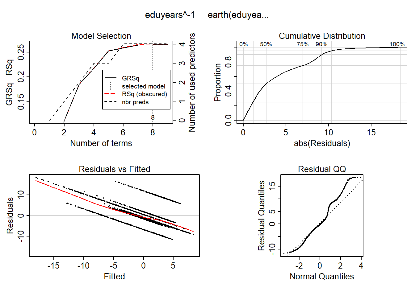
Figure 13: Hockey-stick functions fit with MARS for the predictors, Year 1985 - 2018
plotmo (mmod_scale)## plotmo grid: sum_pop sum_edu_region_year year_n perc_women age_n
## 0.08635757 -0.3683495 -0.04979415 0.1299828 0.2792169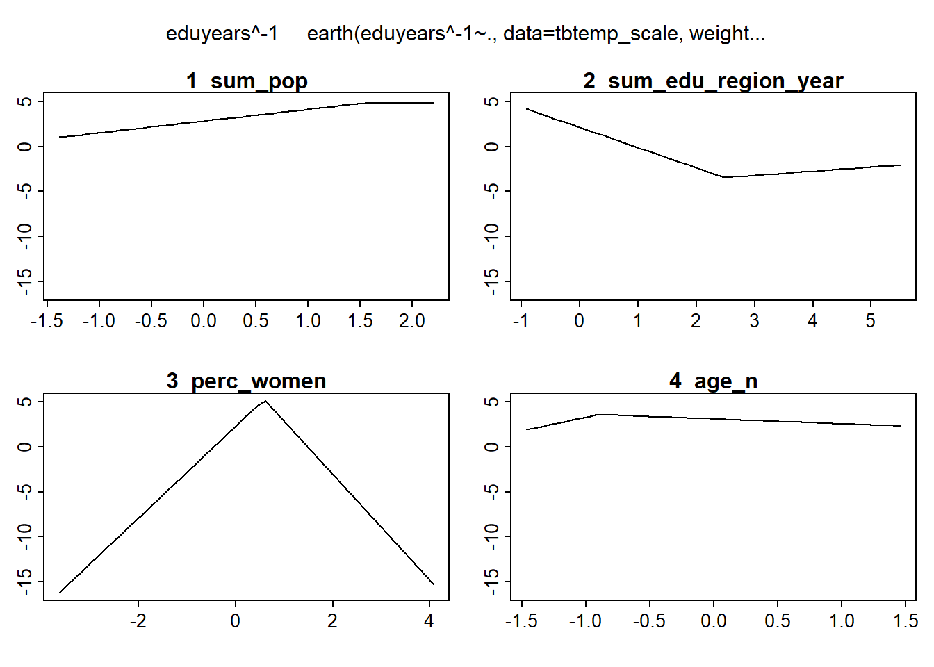
Figure 14: Hockey-stick functions fit with MARS for the predictors, Year 1985 - 2018
model_mmod_scale <- lm (eduyears^-1 ~
  lspline(sum_pop, c(1.54673)) +
  lspline(sum_edu_region_year, c(2.48479)) +
  lspline(perc_women, c(0.589918)) +
  lspline(age_n, c(-0.905736)),
  weights = tbtest$sum_edu_region_year,
  data = tbtemp_scale)

summary (model_mmod_scale)$r.squared
## [1] 0.2657429anova (model_mmod_scale)## Analysis of Variance Table
##
## Response: eduyears^-1
## Df Sum Sq Mean Sq F value
## lspline(sum_pop, c(1.54673)) 2 22976857 11488429 29.585
## lspline(sum_edu_region_year, c(2.48479)) 2 824771527 412385764 1061.981
## lspline(perc_women, c(0.589918)) 2 2195580032 1097790016 2827.043
## lspline(age_n, c(-0.905736)) 2 140046090 70023045 180.324
## Residuals 22651 8795778088 388317
## Pr(>F)
## lspline(sum_pop, c(1.54673)) 1.473e-13 ***
## lspline(sum_edu_region_year, c(2.48479)) < 2.2e-16 ***
## lspline(perc_women, c(0.589918)) < 2.2e-16 ***
## lspline(age_n, c(-0.905736)) < 2.2e-16 ***
## Residuals
## ---
## Signif. codes: 0 '***' 0.001 '**' 0.01 '*' 0.05 '.' 0.1 ' ' 1I will use regsubsets to find the model which minimises the AIC using the standardised data. I will include some plots for diagnostic purposes. I have also included a bootstrap test since we can’t count on the errors to be normally distributed.
b <- regsubsets (eduyears^-1 ~ (lspline(sum_edu_region_year, c(2.48479)) + lspline(perc_women, c(0.589918)) + lspline(age_n, c(-0.905736)) + year_n + lspline(sum_pop, c(1.54673))) * (lspline(sum_edu_region_year, c(2.48479)) + lspline(perc_women, c(0.589918)) + lspline(age_n, c(-0.905736)) + year_n + lspline(sum_pop, c(1.54673))), weights = tbnum$sum_edu_region_year, data = tbtemp_scale, nvmax = 12)

rs <- summary(b)
AIC <- 50 * log (rs$rss / 50) + (2:13) * 2
which.min (AIC)
## [1] 4names (rs$which[4,])[rs$which[4,]]## [1] "(Intercept)"
## [2] "lspline(perc_women, c(0.589918))1"
## [3] "lspline(sum_edu_region_year, c(2.48479))1:lspline(age_n, c(-0.905736))1"
## [4] "lspline(perc_women, c(0.589918))2:lspline(age_n, c(-0.905736))2"
## [5] "lspline(age_n, c(-0.905736))1:lspline(sum_pop, c(1.54673))1"model <- lm (eduyears^-1 ~
lspline(perc_women, c(0.402156)) +
lspline(sum_edu_region_year, c(68923)):lspline(age_n, c(29.5)) +
lspline(perc_women, c(0.402156)):lspline(age_n, c(29.5)) +
lspline(age_n, c(29.5)):sum_pop,
weights = tbnum$sum_edu_region_year,
data = tbnum)
boxcox(model)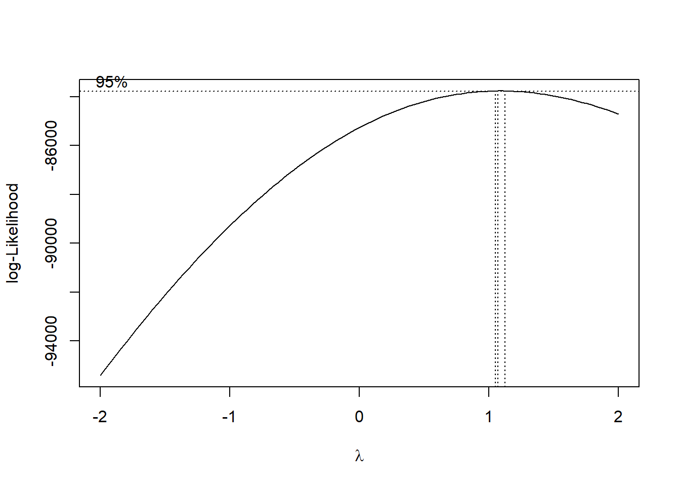
Figure 15: Find the model that minimises the AIC, Year 1985 - 2018
summary (model)##
## Call:
## lm(formula = eduyears^-1 ~ lspline(perc_women, c(0.402156)) +
## lspline(sum_edu_region_year, c(68923)):lspline(age_n, c(29.5)) +
## lspline(perc_women, c(0.402156)):lspline(age_n, c(29.5)) +
## lspline(age_n, c(29.5)):sum_pop, data = tbnum, weights = tbnum$sum_edu_region_year)
##
## Weighted Residuals:
## Min 1Q Median 3Q Max
## -7.7236 -1.3350 -0.2622 1.2344 6.2808
##
## Coefficients:
## Estimate
## (Intercept) 6.003e-02
## lspline(perc_women, c(0.402156))1 1.614e-01
## lspline(perc_women, c(0.402156))2 -9.712e-02
## lspline(sum_edu_region_year, c(68923))1:lspline(age_n, c(29.5))1 1.680e-09
## lspline(sum_edu_region_year, c(68923))2:lspline(age_n, c(29.5))1 -9.445e-10
## lspline(sum_edu_region_year, c(68923))1:lspline(age_n, c(29.5))2 1.449e-08
## lspline(sum_edu_region_year, c(68923))2:lspline(age_n, c(29.5))2 -1.359e-10
## lspline(perc_women, c(0.402156))1:lspline(age_n, c(29.5))1 -1.611e-03
## lspline(perc_women, c(0.402156))2:lspline(age_n, c(29.5))1 -2.570e-03
## lspline(perc_women, c(0.402156))1:lspline(age_n, c(29.5))2 1.802e-04
## lspline(perc_women, c(0.402156))2:lspline(age_n, c(29.5))2 3.535e-03
## lspline(age_n, c(29.5))1:sum_pop -2.162e-10
## lspline(age_n, c(29.5))2:sum_pop -3.873e-10
## Std. Error
## (Intercept) 1.629e-03
## lspline(perc_women, c(0.402156))1 6.578e-03
## lspline(perc_women, c(0.402156))2 2.087e-02
## lspline(sum_edu_region_year, c(68923))1:lspline(age_n, c(29.5))1 3.435e-10
## lspline(sum_edu_region_year, c(68923))2:lspline(age_n, c(29.5))1 6.753e-10
## lspline(sum_edu_region_year, c(68923))1:lspline(age_n, c(29.5))2 4.415e-10
## lspline(sum_edu_region_year, c(68923))2:lspline(age_n, c(29.5))2 1.118e-09
## lspline(perc_women, c(0.402156))1:lspline(age_n, c(29.5))1 1.893e-04
## lspline(perc_women, c(0.402156))2:lspline(age_n, c(29.5))1 7.417e-04
## lspline(perc_women, c(0.402156))1:lspline(age_n, c(29.5))2 6.717e-05
## lspline(perc_women, c(0.402156))2:lspline(age_n, c(29.5))2 1.212e-04
## lspline(age_n, c(29.5))1:sum_pop 1.854e-11
## lspline(age_n, c(29.5))2:sum_pop 2.233e-11
## t value
## (Intercept) 36.838
## lspline(perc_women, c(0.402156))1 24.541
## lspline(perc_women, c(0.402156))2 -4.653
## lspline(sum_edu_region_year, c(68923))1:lspline(age_n, c(29.5))1 4.890
## lspline(sum_edu_region_year, c(68923))2:lspline(age_n, c(29.5))1 -1.399
## lspline(sum_edu_region_year, c(68923))1:lspline(age_n, c(29.5))2 32.817
## lspline(sum_edu_region_year, c(68923))2:lspline(age_n, c(29.5))2 -0.122
## lspline(perc_women, c(0.402156))1:lspline(age_n, c(29.5))1 -8.510
## lspline(perc_women, c(0.402156))2:lspline(age_n, c(29.5))1 -3.465
## lspline(perc_women, c(0.402156))1:lspline(age_n, c(29.5))2 2.683
## lspline(perc_women, c(0.402156))2:lspline(age_n, c(29.5))2 29.180
## lspline(age_n, c(29.5))1:sum_pop -11.660
## lspline(age_n, c(29.5))2:sum_pop -17.345
## Pr(>|t|)
## (Intercept) < 2e-16 ***
## lspline(perc_women, c(0.402156))1 < 2e-16 ***
## lspline(perc_women, c(0.402156))2 3.30e-06 ***
## lspline(sum_edu_region_year, c(68923))1:lspline(age_n, c(29.5))1 1.01e-06 ***
## lspline(sum_edu_region_year, c(68923))2:lspline(age_n, c(29.5))1 0.161945
## lspline(sum_edu_region_year, c(68923))1:lspline(age_n, c(29.5))2 < 2e-16 ***
## lspline(sum_edu_region_year, c(68923))2:lspline(age_n, c(29.5))2 0.903193
## lspline(perc_women, c(0.402156))1:lspline(age_n, c(29.5))1 < 2e-16 ***
## lspline(perc_women, c(0.402156))2:lspline(age_n, c(29.5))1 0.000531 ***
## lspline(perc_women, c(0.402156))1:lspline(age_n, c(29.5))2 0.007309 **
## lspline(perc_women, c(0.402156))2:lspline(age_n, c(29.5))2 < 2e-16 ***
## lspline(age_n, c(29.5))1:sum_pop < 2e-16 ***
## lspline(age_n, c(29.5))2:sum_pop < 2e-16 ***
## ---
## Signif. codes: 0 '***' 0.001 '**' 0.01 '*' 0.05 '.' 0.1 ' ' 1
##
## Residual standard error: 2.069 on 22647 degrees of freedom
## Multiple R-squared: 0.3847, Adjusted R-squared: 0.3844
## F-statistic: 1180 on 12 and 22647 DF, p-value: < 2.2e-16anova (model)## Analysis of Variance Table
##
## Response: eduyears^-1
## Df Sum Sq
## lspline(perc_women, c(0.402156)) 2 13795
## lspline(sum_edu_region_year, c(68923)):lspline(age_n, c(29.5)) 4 29033
## lspline(perc_women, c(0.402156)):lspline(age_n, c(29.5)) 4 8736
## lspline(age_n, c(29.5)):sum_pop 2 9027
## Residuals 22647 96916
## Mean Sq F value
## lspline(perc_women, c(0.402156)) 6897.3 1611.75
## lspline(sum_edu_region_year, c(68923)):lspline(age_n, c(29.5)) 7258.3 1696.10
## lspline(perc_women, c(0.402156)):lspline(age_n, c(29.5)) 2183.9 510.33
## lspline(age_n, c(29.5)):sum_pop 4513.4 1054.67
## Residuals 4.3
## Pr(>F)
## lspline(perc_women, c(0.402156)) < 2.2e-16 ***
## lspline(sum_edu_region_year, c(68923)):lspline(age_n, c(29.5)) < 2.2e-16 ***
## lspline(perc_women, c(0.402156)):lspline(age_n, c(29.5)) < 2.2e-16 ***
## lspline(age_n, c(29.5)):sum_pop < 2.2e-16 ***
## Residuals
## ---
## Signif. codes: 0 '***' 0.001 '**' 0.01 '*' 0.05 '.' 0.1 ' ' 1plot (model)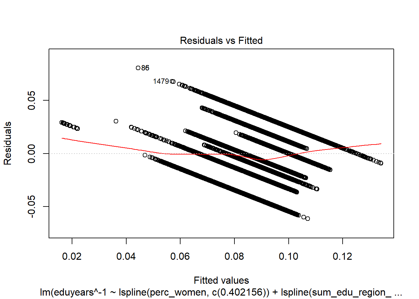
Figure 16: Find the model that minimises the AIC, Year 1985 - 2018
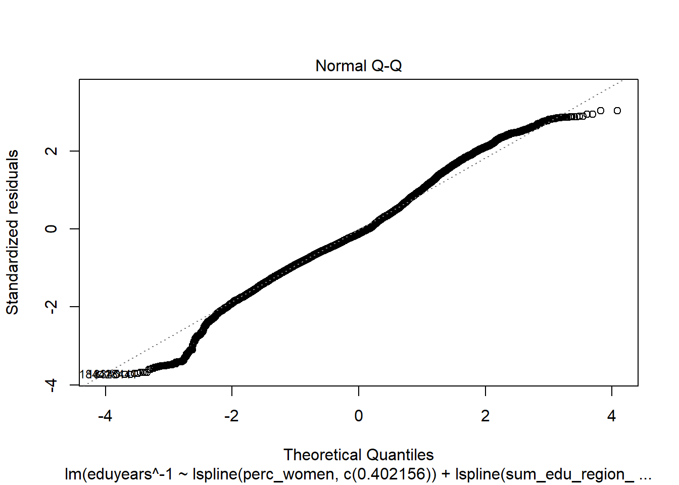
Figure 17: Find the model that minimises the AIC, Year 1985 - 2018
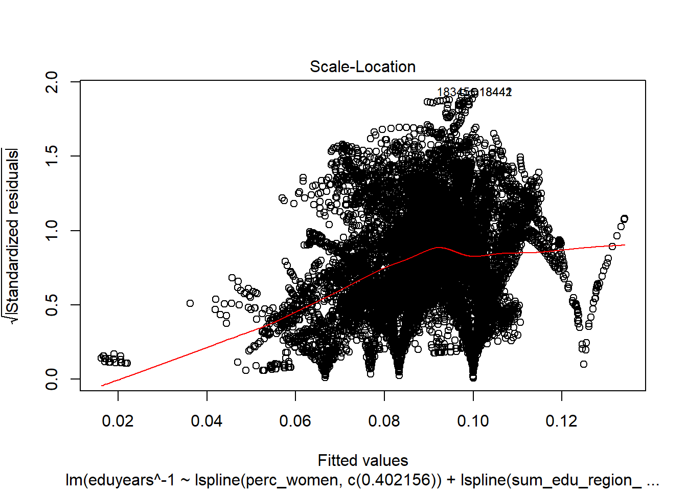
Figure 18: Find the model that minimises the AIC, Year 1985 - 2018
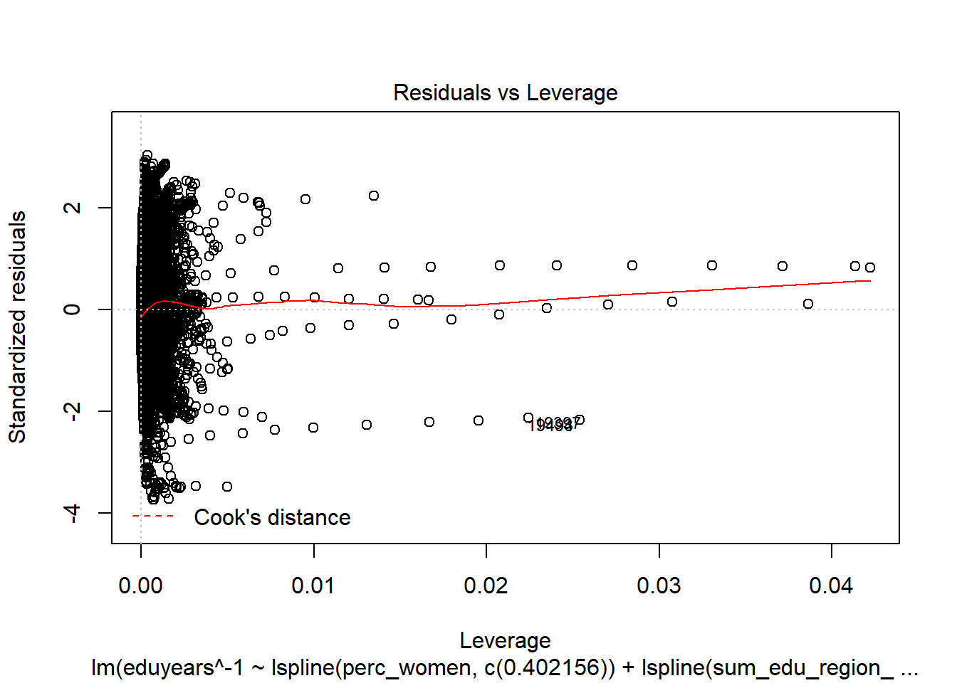
Figure 19: Find the model that minimises the AIC, Year 1985 - 2018
binnedplot(predict(model), resid(model))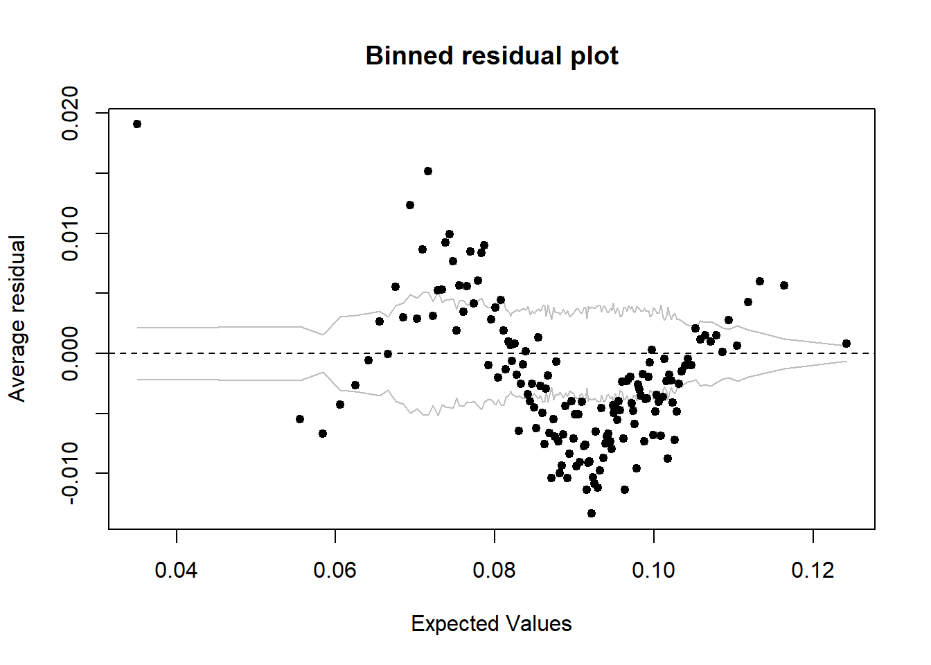
Figure 20: Find the model that minimises the AIC, Year 1985 - 2018
halfnorm(rstudent(model))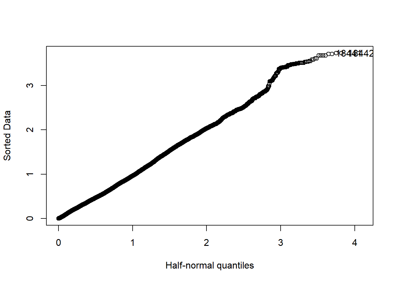
Figure 21: Find the model that minimises the AIC, Year 1985 - 2018
tbnum %>% mutate(residuals = residuals(model)) %>%
  group_by(eduyears, region, year_n, age_n) %>%
  summarise(residuals = mean(residuals), count = sum(groupsize)) %>%
    ggplot (aes(x = eduyears, y = residuals, size = sqrt(count), colour = year_n)) +
    geom_point() + facet_grid(. ~ age_n)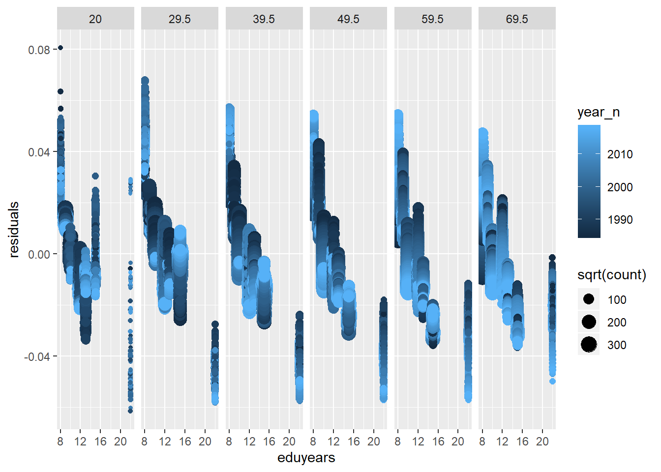
Figure 22: Find the model that minimises the AIC, Year 1985 - 2018
tbnumpred <- bind_cols(tbnum, as_tibble(predict(model, tbnum, interval = "confidence")))

suppressWarnings(multiclass.roc(tbnumpred$eduyears, tbnumpred$fit))
## Setting direction: controls > cases## Setting direction: controls < cases## Setting direction: controls > cases
## Setting direction: controls > cases
## Setting direction: controls > cases
## Setting direction: controls > cases## Setting direction: controls < cases## Setting direction: controls > cases
## Setting direction: controls > cases
## Setting direction: controls > cases
## Setting direction: controls > cases
## Setting direction: controls > cases
## Setting direction: controls > cases
## Setting direction: controls > cases
## Setting direction: controls > cases
## Setting direction: controls > cases
## Setting direction: controls > cases
## Setting direction: controls > cases
## Setting direction: controls > cases
## Setting direction: controls > cases
## Setting direction: controls > cases##
## Call:
## multiclass.roc.default(response = tbnumpred$eduyears, predictor = tbnumpred$fit)
##
## Data: tbnumpred$fit with 7 levels of tbnumpred$eduyears: 8, 9, 10, 12, 13, 15, 22.
## Multi-class area under the curve: 0.6936bs <- function(formula, data, indices) {
d <- data[indices,] # allows boot to select sample
fit <- lm(formula, weights = sum_edu_region_year, data=d)
return(coef(fit))
}
results <- boot(data = tbnum, statistic = bs,
R = 1000, formula = eduyears^-1 ~
lspline(perc_women, c(0.402156)) +
lspline(sum_edu_region_year, c(68923)):lspline(age_n, c(29.5)) +
lspline(perc_women, c(0.402156)):lspline(age_n, c(29.5)) +
lspline(age_n, c(29.5)):sum_pop,
weights = tbnum$sum_edu_region_year)
results##
## WEIGHTED BOOTSTRAP
##
##
## Call:
## boot(data = tbnum, statistic = bs, R = 1000, weights = tbnum$sum_edu_region_year,
## formula = eduyears^-1 ~ lspline(perc_women, c(0.402156)) +
## lspline(sum_edu_region_year, c(68923)):lspline(age_n,
## c(29.5)) + lspline(perc_women, c(0.402156)):lspline(age_n,
## c(29.5)) + lspline(age_n, c(29.5)):sum_pop)
##
##
## Bootstrap Statistics :
## original bias std. error mean(t*)
## t1* 6.002560e-02 6.282966e-03 1.487621e-03 6.630857e-02
## t2* 1.614448e-01 -1.489491e-02 6.393635e-03 1.465499e-01
## t3* -9.712093e-02 7.221993e-02 1.927104e-02 -2.490101e-02
## t4* 1.679729e-09 4.440291e-09 3.270648e-10 6.120020e-09
## t5* -9.444671e-10 1.440855e-10 3.744453e-10 -8.003816e-10
## t6* 1.448852e-08 -3.952505e-09 4.193252e-10 1.053602e-08
## t7* -1.359400e-10 1.468111e-09 5.529310e-10 1.332171e-09
## t8* -1.610831e-03 6.882804e-05 1.801159e-04 -1.542003e-03
## t9* -2.570250e-03 -2.067477e-03 6.732789e-04 -4.637727e-03
## t10* 1.801919e-04 7.229534e-04 6.282813e-05 9.031453e-04
## t11* 3.535199e-03 -1.161393e-03 1.113341e-04 2.373805e-03
## t12* -2.161738e-10 -2.930531e-10 1.634625e-11 -5.092269e-10
## t13* -3.872669e-10 6.108726e-11 2.103217e-11 -3.261797e-10plot(results, index=1) # intercept 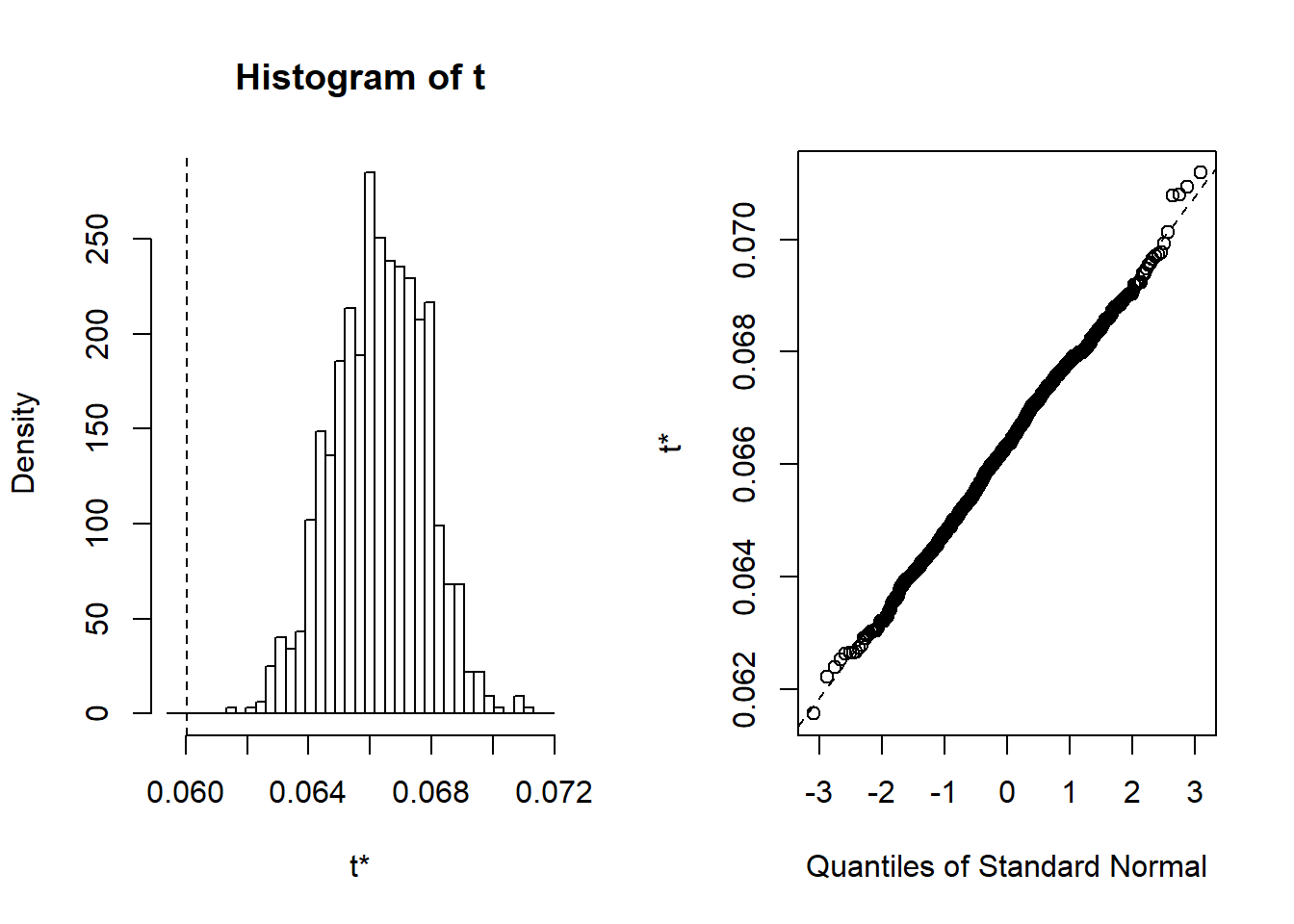
Figure 23: Find the model that minimises the AIC, Year 1985 - 2018
There are a few things I would like to investigate to improve the credibility of the analysis. I will assume that the data can be grouped by year of birth and region and investigate how this will affect the model. I have scaled the weights not to affect the residual standard deviation. I will include some plots for diagnostic purposes. I will assume that each year of birth and each region is a group and set them as random effects and the rest of the predictors as fixed effects. I use the mean age in each age group as the year of birth.
temp <- tbnum %>% mutate(yob = year_n - age_n) %>% mutate(region = tbnum$region)

temp <- data.frame(temp)

weights_scaled <- tbtest$sum_edu_region_year / max(tbtest$sum_edu_region_year)

mmodel <- lmer (eduyears^-1 ~
   lspline(perc_women, c(0.402156)) +
   lspline(sum_edu_region_year, c(68923)):lspline(age_n, c(29.5)) +
   lspline(perc_women, c(0.402156)):lspline(age_n, c(29.5)) +
   lspline(age_n, c(29.5)):sum_pop +
   (1|yob) +
   (1|region),
   weights = weights_scaled,
   data = temp)
## Warning: Some predictor variables are on very different scales: consider
## rescalingplot(mmodel)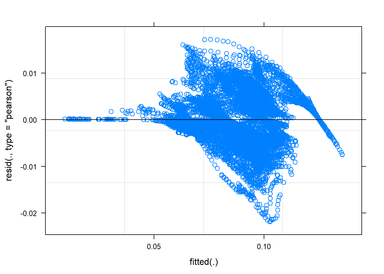
Figure 24: A diagnostic plot of the model with random effects components
qqnorm (residuals(mmodel), main="")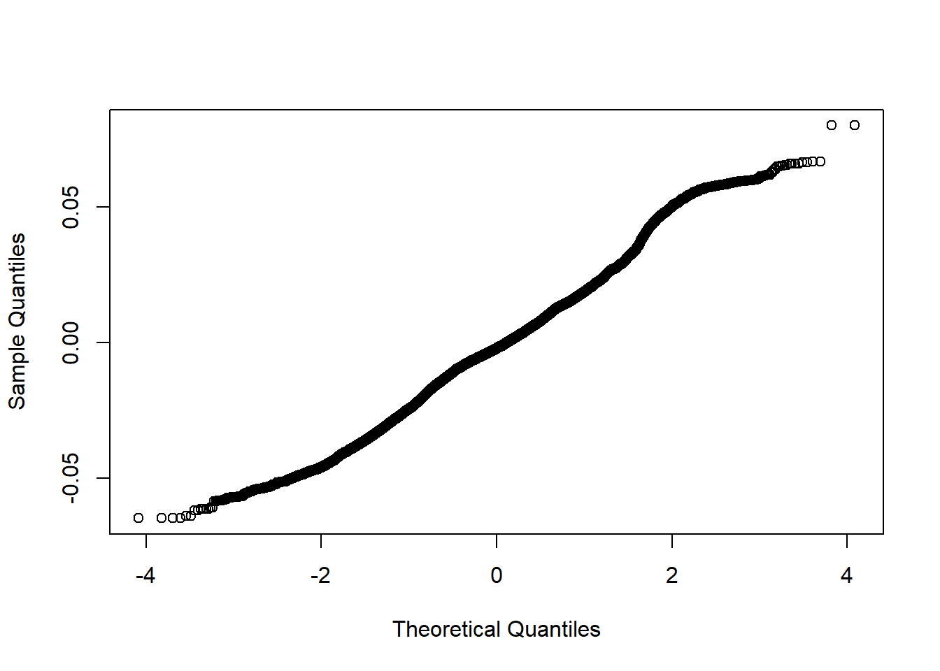
Figure 25: A diagnostic plot of the model with random effects components
summary (mmodel)## Linear mixed model fit by REML ['lmerMod']
## Formula:
## eduyears^-1 ~ lspline(perc_women, c(0.402156)) + lspline(sum_edu_region_year,
## c(68923)):lspline(age_n, c(29.5)) + lspline(perc_women, c(0.402156)):lspline(age_n,
## c(29.5)) + lspline(age_n, c(29.5)):sum_pop + (1 | yob) + (1 | region)
## Data: temp
## Weights: weights_scaled
##
## REML criterion at convergence: -107912.7
##
## Scaled residuals:
## Min 1Q Median 3Q Max
## -4.1769 -0.6147 -0.1003 0.6108 3.2800
##
## Random effects:
## Groups Name Variance Std.Dev.
## yob (Intercept) 1.053e-04 0.0102603
## region (Intercept) 8.113e-07 0.0009007
## Residual 2.753e-05 0.0052472
## Number of obs: 22660, groups: yob, 108; region, 8
##
## Fixed effects:
## Estimate
## (Intercept) 3.382e-02
## lspline(perc_women, c(0.402156))1 1.806e-01
## lspline(perc_women, c(0.402156))2 -1.222e-01
## lspline(sum_edu_region_year, c(68923))1:lspline(age_n, c(29.5))1 3.692e-10
## lspline(sum_edu_region_year, c(68923))2:lspline(age_n, c(29.5))1 1.706e-09
## lspline(sum_edu_region_year, c(68923))1:lspline(age_n, c(29.5))2 1.440e-08
## lspline(sum_edu_region_year, c(68923))2:lspline(age_n, c(29.5))2 -5.056e-09
## lspline(perc_women, c(0.402156))1:lspline(age_n, c(29.5))1 8.518e-04
## lspline(perc_women, c(0.402156))2:lspline(age_n, c(29.5))1 -1.818e-03
## lspline(perc_women, c(0.402156))1:lspline(age_n, c(29.5))2 -1.046e-03
## lspline(perc_women, c(0.402156))2:lspline(age_n, c(29.5))2 2.786e-03
## lspline(age_n, c(29.5))1:sum_pop -1.412e-10
## lspline(age_n, c(29.5))2:sum_pop -3.426e-10
## Std. Error
## (Intercept) 2.092e-03
## lspline(perc_women, c(0.402156))1 1.757e-02
## lspline(perc_women, c(0.402156))2 1.953e-02
## lspline(sum_edu_region_year, c(68923))1:lspline(age_n, c(29.5))1 3.244e-10
## lspline(sum_edu_region_year, c(68923))2:lspline(age_n, c(29.5))1 6.564e-10
## lspline(sum_edu_region_year, c(68923))1:lspline(age_n, c(29.5))2 4.148e-10
## lspline(sum_edu_region_year, c(68923))2:lspline(age_n, c(29.5))2 1.112e-09
## lspline(perc_women, c(0.402156))1:lspline(age_n, c(29.5))1 5.885e-04
## lspline(perc_women, c(0.402156))2:lspline(age_n, c(29.5))1 6.941e-04
## lspline(perc_women, c(0.402156))1:lspline(age_n, c(29.5))2 6.737e-05
## lspline(perc_women, c(0.402156))2:lspline(age_n, c(29.5))2 1.167e-04
## lspline(age_n, c(29.5))1:sum_pop 3.051e-11
## lspline(age_n, c(29.5))2:sum_pop 2.143e-11
## t value
## (Intercept) 16.167
## lspline(perc_women, c(0.402156))1 10.280
## lspline(perc_women, c(0.402156))2 -6.258
## lspline(sum_edu_region_year, c(68923))1:lspline(age_n, c(29.5))1 1.138
## lspline(sum_edu_region_year, c(68923))2:lspline(age_n, c(29.5))1 2.599
## lspline(sum_edu_region_year, c(68923))1:lspline(age_n, c(29.5))2 34.716
## lspline(sum_edu_region_year, c(68923))2:lspline(age_n, c(29.5))2 -4.549
## lspline(perc_women, c(0.402156))1:lspline(age_n, c(29.5))1 1.448
## lspline(perc_women, c(0.402156))2:lspline(age_n, c(29.5))1 -2.619
## lspline(perc_women, c(0.402156))1:lspline(age_n, c(29.5))2 -15.525
## lspline(perc_women, c(0.402156))2:lspline(age_n, c(29.5))2 23.876
## lspline(age_n, c(29.5))1:sum_pop -4.627
## lspline(age_n, c(29.5))2:sum_pop -15.987##
## Correlation matrix not shown by default, as p = 13 > 12.
## Use print(x, correlation=TRUE) or
## vcov(x) if you need it## fit warnings:
## Some predictor variables are on very different scales: consider rescalinganova (mmodel)## Analysis of Variance Table
## Df Sum Sq
## lspline(perc_women, c(0.402156)) 2 0.243294
## lspline(sum_edu_region_year, c(68923)):lspline(age_n, c(29.5)) 4 0.060730
## lspline(perc_women, c(0.402156)):lspline(age_n, c(29.5)) 4 0.030402
## lspline(age_n, c(29.5)):sum_pop 2 0.014060
## Mean Sq F value
## lspline(perc_women, c(0.402156)) 0.121647 4418.15
## lspline(sum_edu_region_year, c(68923)):lspline(age_n, c(29.5)) 0.015182 551.42
## lspline(perc_women, c(0.402156)):lspline(age_n, c(29.5)) 0.007600 276.04
## lspline(age_n, c(29.5)):sum_pop 0.007030 255.32binnedplot(predict(mmodel), resid(mmodel))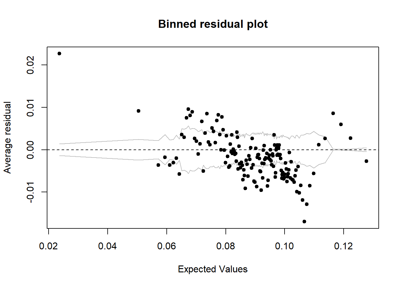
Figure 26: A diagnostic plot of the model with random effects components
halfnorm(rstudent(mmodel))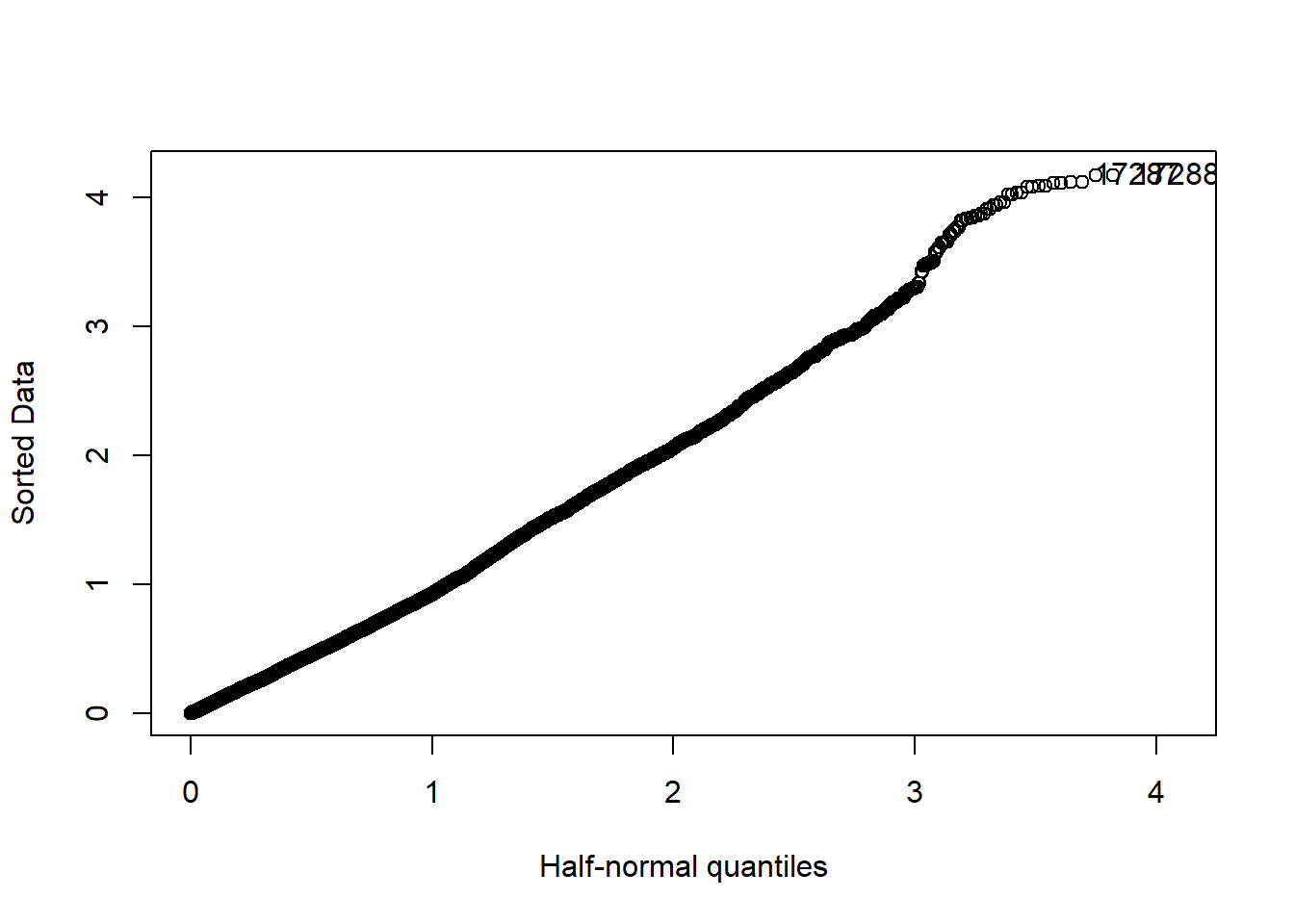
Figure 27: A diagnostic plot of the model with random effects components
tbnum %>% mutate(residuals = residuals(mmodel)) %>%
  group_by(eduyears, region, year_n, age_n) %>%
  summarise(residuals = mean(residuals), count = sum(groupsize)) %>%
    ggplot (aes(x = eduyears, y = residuals, size = sqrt(count), colour = year_n)) +
    geom_point() + facet_grid(. ~ age_n)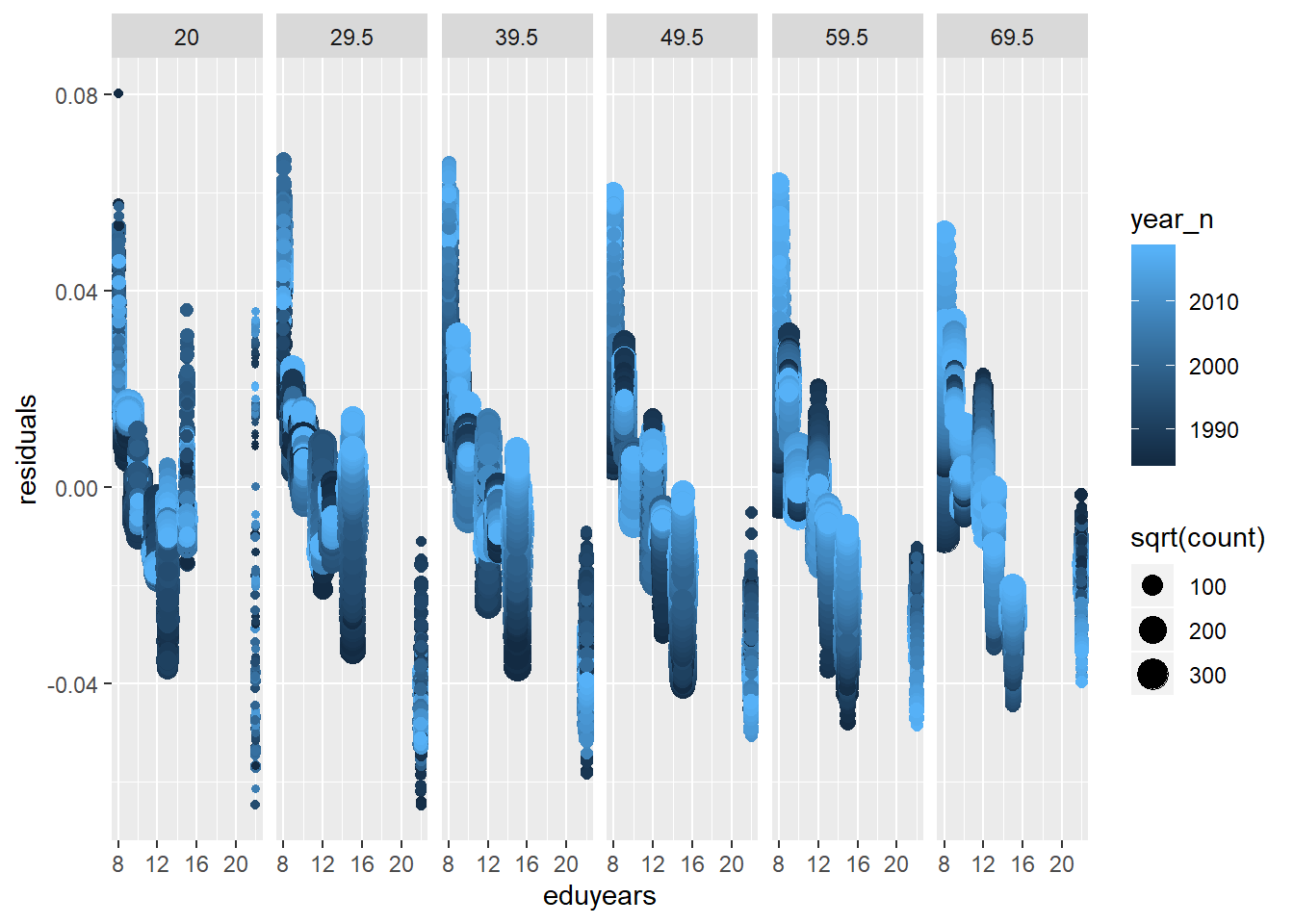
Figure 28: A diagnostic plot of the model with random effects components
tbnumpred <- bind_cols(temp, as_tibble(predict(mmodel, temp, interval = "confidence")))## Warning in predict.merMod(mmodel, temp, interval = "confidence"): unused
## arguments ignored## Warning: Calling `as_tibble()` on a vector is discouraged, because the behavior is likely to change in the future. Use `tibble::enframe(name = NULL)` instead.
## This warning is displayed once per session.suppressWarnings (multiclass.roc (tbnumpred$eduyears, tbnumpred$value))## Setting direction: controls > cases## Setting direction: controls < cases## Setting direction: controls > cases
## Setting direction: controls > cases
## Setting direction: controls > cases
## Setting direction: controls > cases## Setting direction: controls < cases## Setting direction: controls > cases
## Setting direction: controls > cases
## Setting direction: controls > cases
## Setting direction: controls > cases
## Setting direction: controls > cases
## Setting direction: controls > cases
## Setting direction: controls > cases
## Setting direction: controls > cases
## Setting direction: controls > cases
## Setting direction: controls > cases
## Setting direction: controls > cases## Setting direction: controls < cases## Setting direction: controls > cases
## Setting direction: controls > cases##
## Call:
## multiclass.roc.default(response = tbnumpred$eduyears, predictor = tbnumpred$value)
##
## Data: tbnumpred$value with 7 levels of tbnumpred$eduyears: 8, 9, 10, 12, 13, 15, 22.
## Multi-class area under the curve: 0.6939mySumm <- function(.) { s <- sigma(.)
c(beta =getME(., "beta"), sigma = s, sig01 = unname(s * getME(., "theta"))) }
results <- bootMer(mmodel, mySumm, nsim = 1000)
results##
## PARAMETRIC BOOTSTRAP
##
##
## Call:
## bootMer(x = mmodel, FUN = mySumm, nsim = 1000)
##
##
## Bootstrap Statistics :
## original bias std. error
## t1* 3.382171e-02 3.204383e-05 1.370011e-03
## t2* 1.806110e-01 5.656583e-04 1.586369e-02
## t3* -1.222301e-01 -1.200144e-04 7.545495e-03
## t4* 3.692235e-10 1.574681e-11 1.758515e-10
## t5* 1.705945e-09 -8.046354e-12 5.355611e-10
## t6* 1.440064e-08 -1.696450e-11 2.268515e-10
## t7* -5.055769e-09 1.234462e-11 8.717959e-10
## t8* 8.518246e-04 -2.117494e-05 5.396222e-04
## t9* -1.817991e-03 5.758882e-06 2.800208e-04
## t10* -1.045953e-03 1.165115e-06 3.192411e-05
## t11* 2.786456e-03 -8.257204e-08 6.151912e-05
## t12* -1.411911e-10 -7.934184e-13 2.229494e-11
## t13* -3.426241e-10 1.956803e-13 9.642223e-12
## t14* 5.247231e-03 -3.268970e-03 1.377226e-05
## t15* 1.026026e-02 -6.487712e-06 6.957391e-04
## t16* 9.007187e-04 -1.190123e-05 2.607631e-04##
## 118 warning(s): Model failed to converge with max|grad| = 0.00200096 (tol = 0.002, component 1) (and others)plot(results)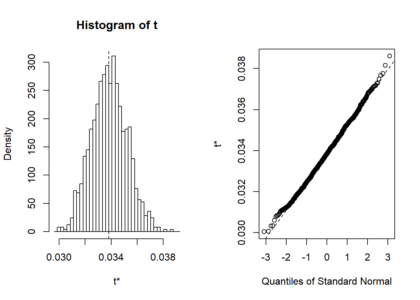
Figure 29: A diagnostic plot of the model with random effects components
Now let’s see what we have found. I will plot all the models for comparison. I could not get the back transformation in sjPlot to work for the response variable so you will have to endure that the response is the inverse of years of education.
transformeddata <- tbnum %>%  mutate(eduyears = eduyears ^ -1)

model <- lm (eduyears ~
   lspline(perc_women, c(0.402156)) +
   lspline(sum_edu_region_year, c(68923)):lspline(age_n, c(29.5)) +
   lspline(perc_women, c(0.402156)):lspline(age_n, c(29.5)) +
   lspline(age_n, c(29.5)):sum_pop,
   weights = tbnum$sum_edu_region_year,
   data = transformeddata)

temp <- transformeddata %>% mutate(yob = year_n - age_n) %>% mutate(region = tbnum$region)

temp <- data.frame(temp)

mmodel <- lmer (eduyears ~
   lspline(perc_women, c(0.402156)) +
   lspline(sum_edu_region_year, c(68923)):lspline(age_n, c(29.5)) +
   lspline(perc_women, c(0.402156)):lspline(age_n, c(29.5)) +
   lspline(age_n, c(29.5)):sum_pop +
   (1|yob) +
   (1|region),
   weights = weights_scaled,
   data = temp)
## Warning: Some predictor variables are on very different scales: consider
## rescalingplot_model (model, type = "pred", terms = c("perc_women"))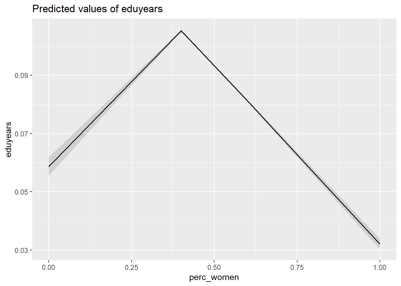
Figure 30: The significance of the per cent women on the level of education, Year 1985 - 2018
plot_model (mmodel, type = "pred", terms = c("perc_women"))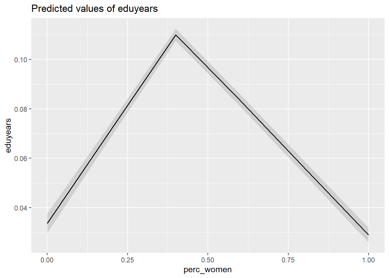
Figure 31: The significance of the per cent women on the level of education, Year 1985 - 2018
tbnum %>%
  ggplot () +
    geom_jitter (mapping = aes(x = perc_women, y = eduyears )) +
  labs(
    x = "Per cent women",
    y = "Years of education"
  )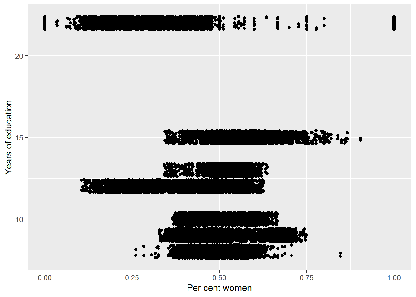
Figure 32: The significance of the per cent women on the level of education, Year 1985 - 2018
plot_model (model, type = "pred", terms = c("age_n", "sum_edu_region_year"))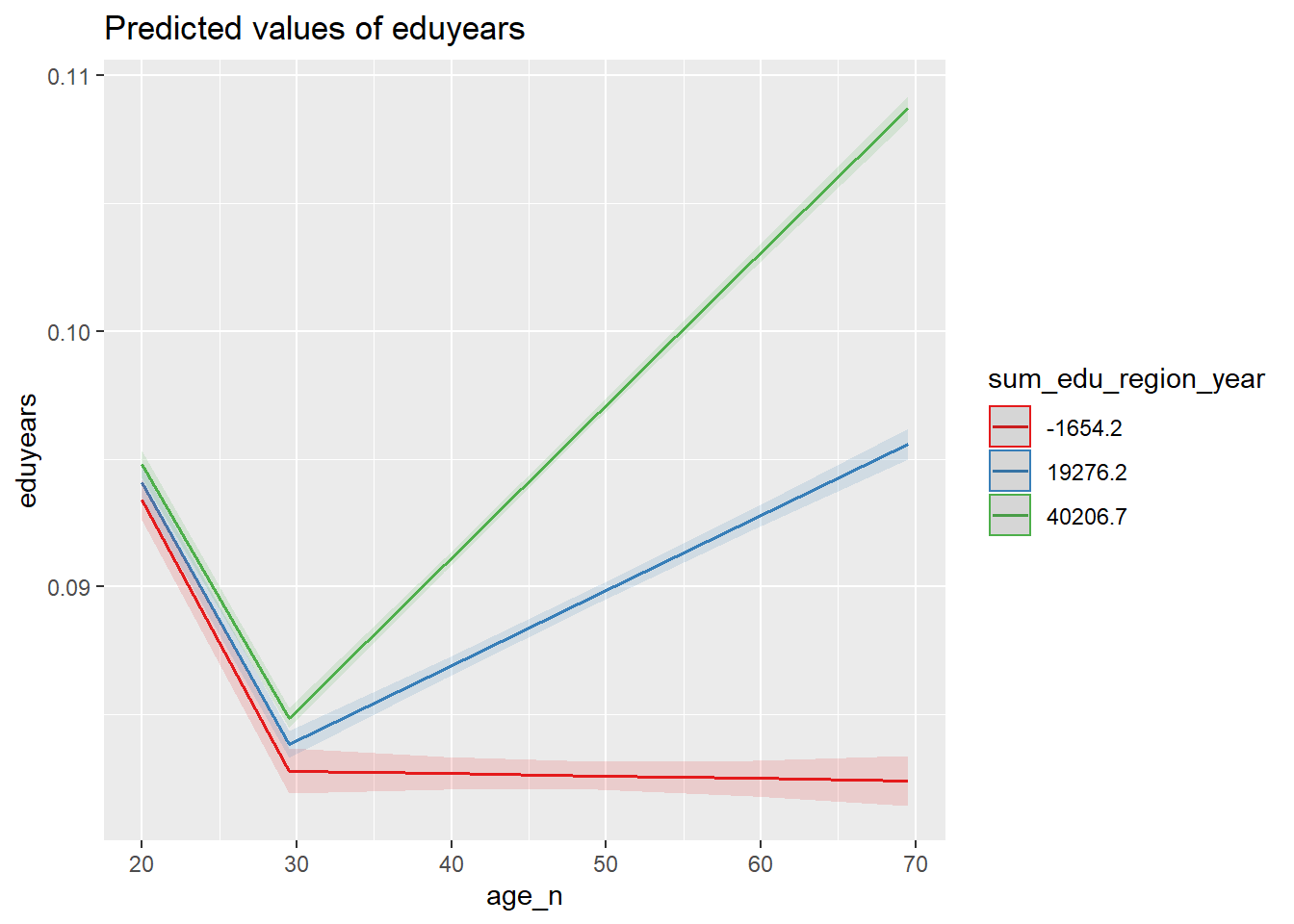
Figure 33: The significance of the interaction between the number of persons with the same level of education, region and year, age and age on the level of education, Year 1985 - 2018
plot_model (mmodel, type = "pred", terms = c("age_n", "sum_edu_region_year"))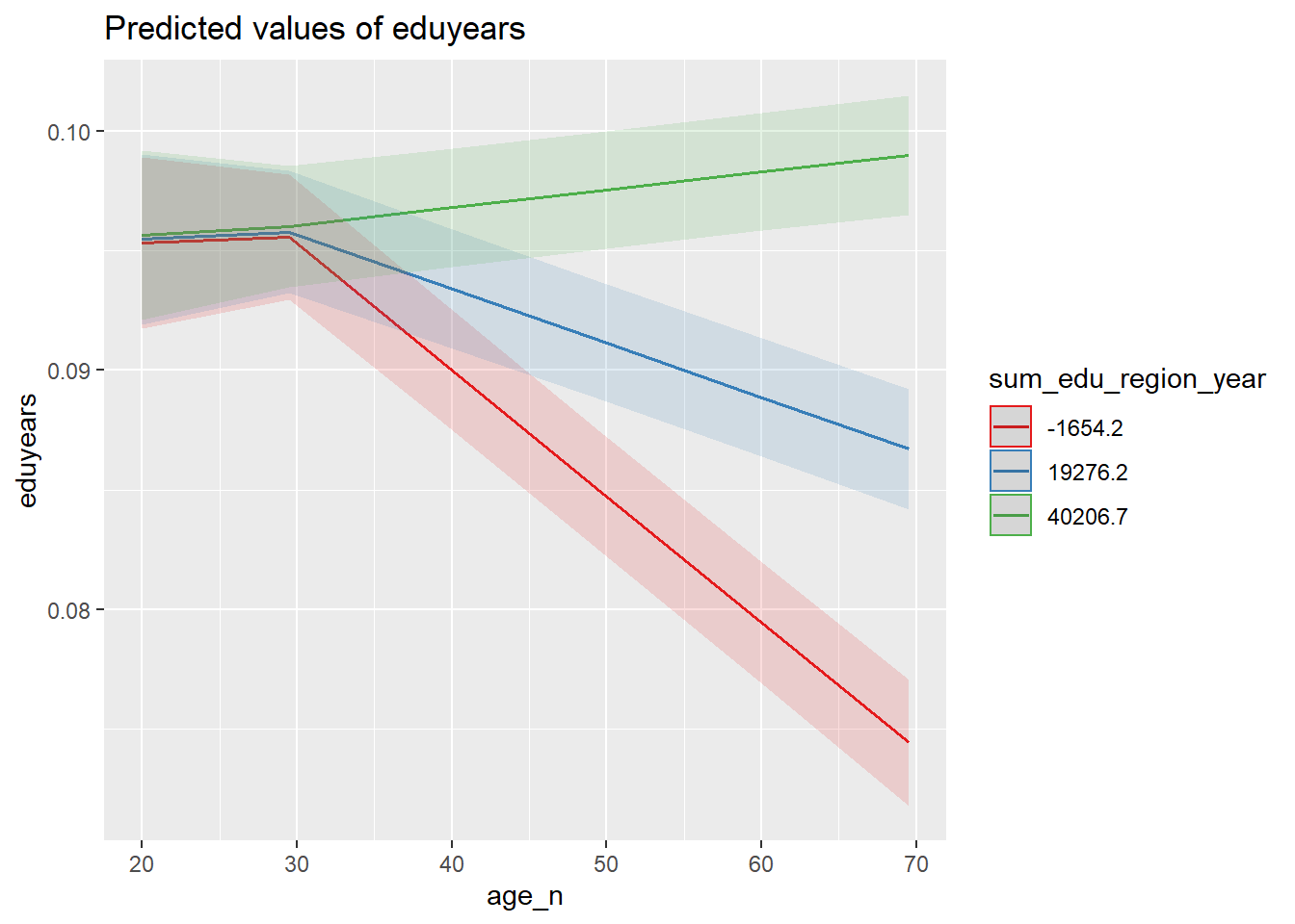
Figure 34: The significance of the interaction between the number of persons with the same level of education, region and year, age and age on the level of education, Year 1985 - 2018
tbnum %>%
  ggplot () +
    geom_jitter (mapping = aes(x = sum_edu_region_year, y = eduyears, colour = age_n)) +
  labs(
    x = "# persons with same edulevel, region, year, age",
    y = "Years of education"
  )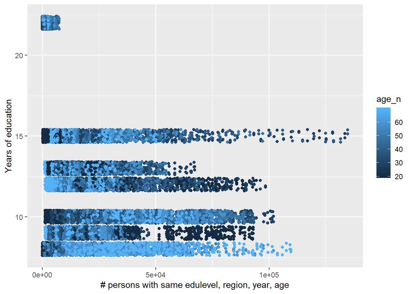
Figure 35: The significance of the interaction between the number of persons with the same level of education, region and year, age and age on the level of education, Year 1985 - 2018
plot_model (model, type = "pred", terms = c("age_n", "perc_women"))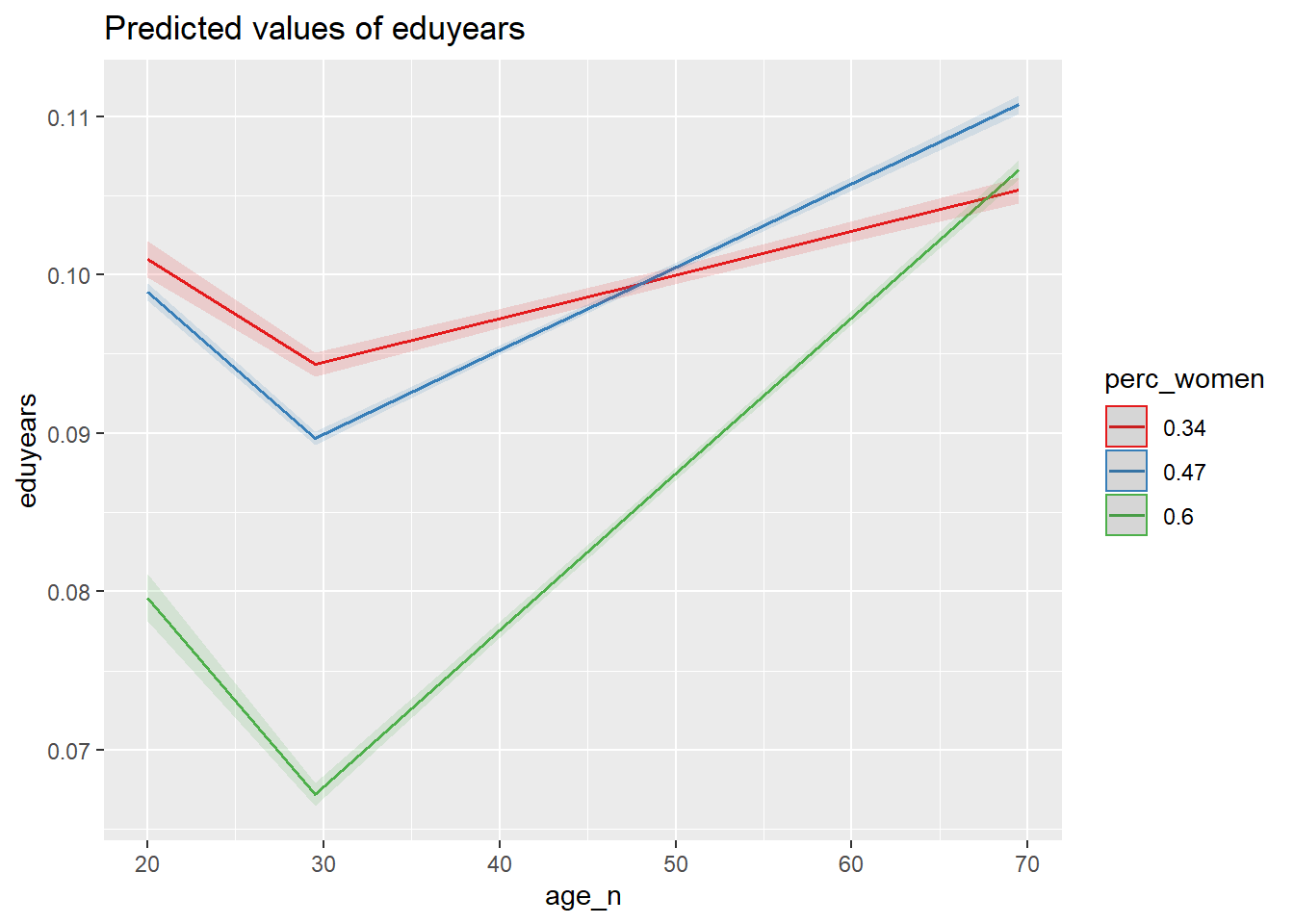
Figure 36: The significance of the interaction between per cent women and age on the level of education, Year 1985 - 2018
plot_model (mmodel, type = "pred", terms = c("age_n", "perc_women"))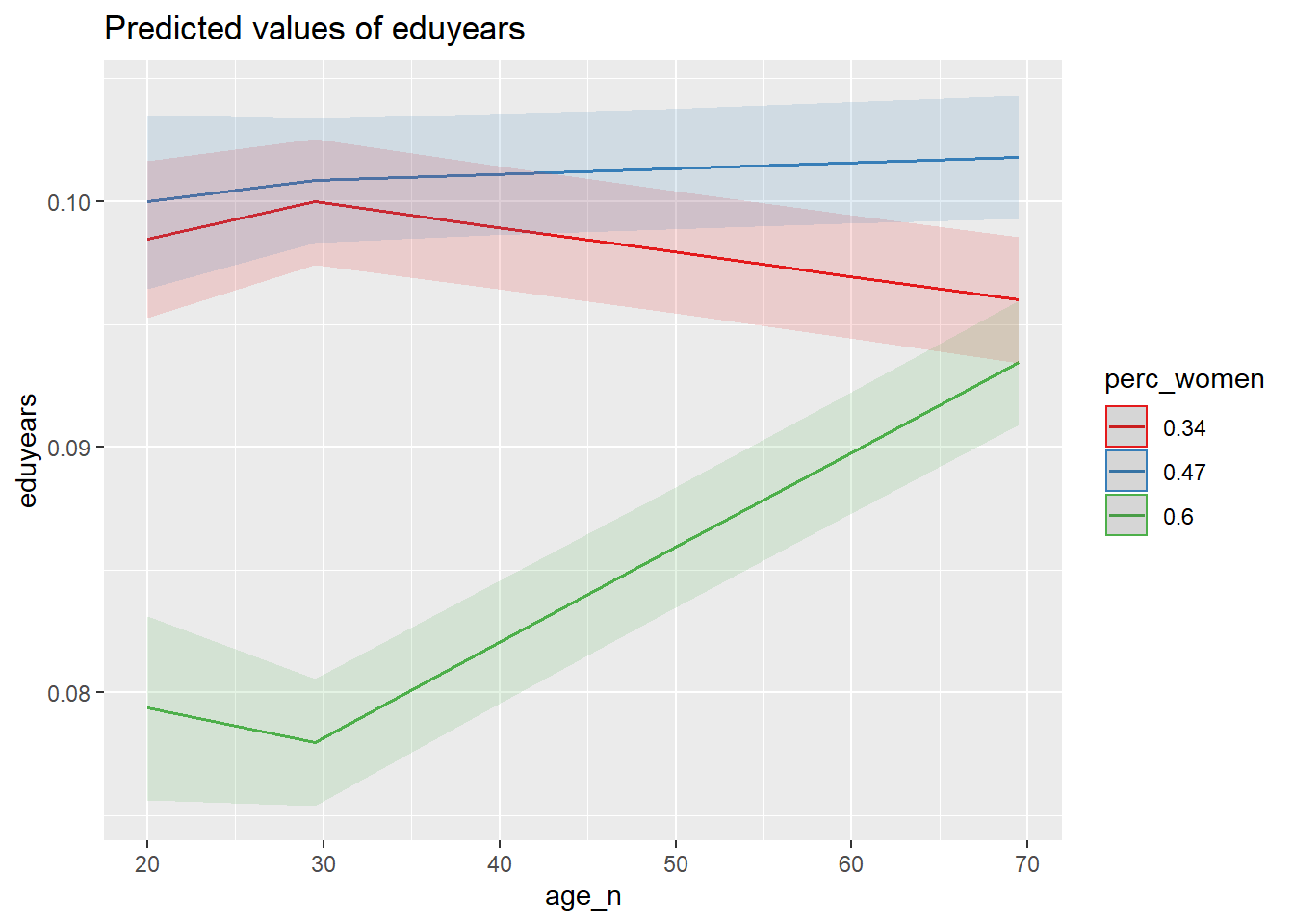
Figure 37: The significance of the interaction between per cent women and age on the level of education, Year 1985 - 2018
tbnum %>%
  ggplot () +
    geom_jitter (mapping = aes(x = perc_women, y = eduyears, colour = age_n)) +
  labs(
    x = "Age",
    y = "Years of education"
  )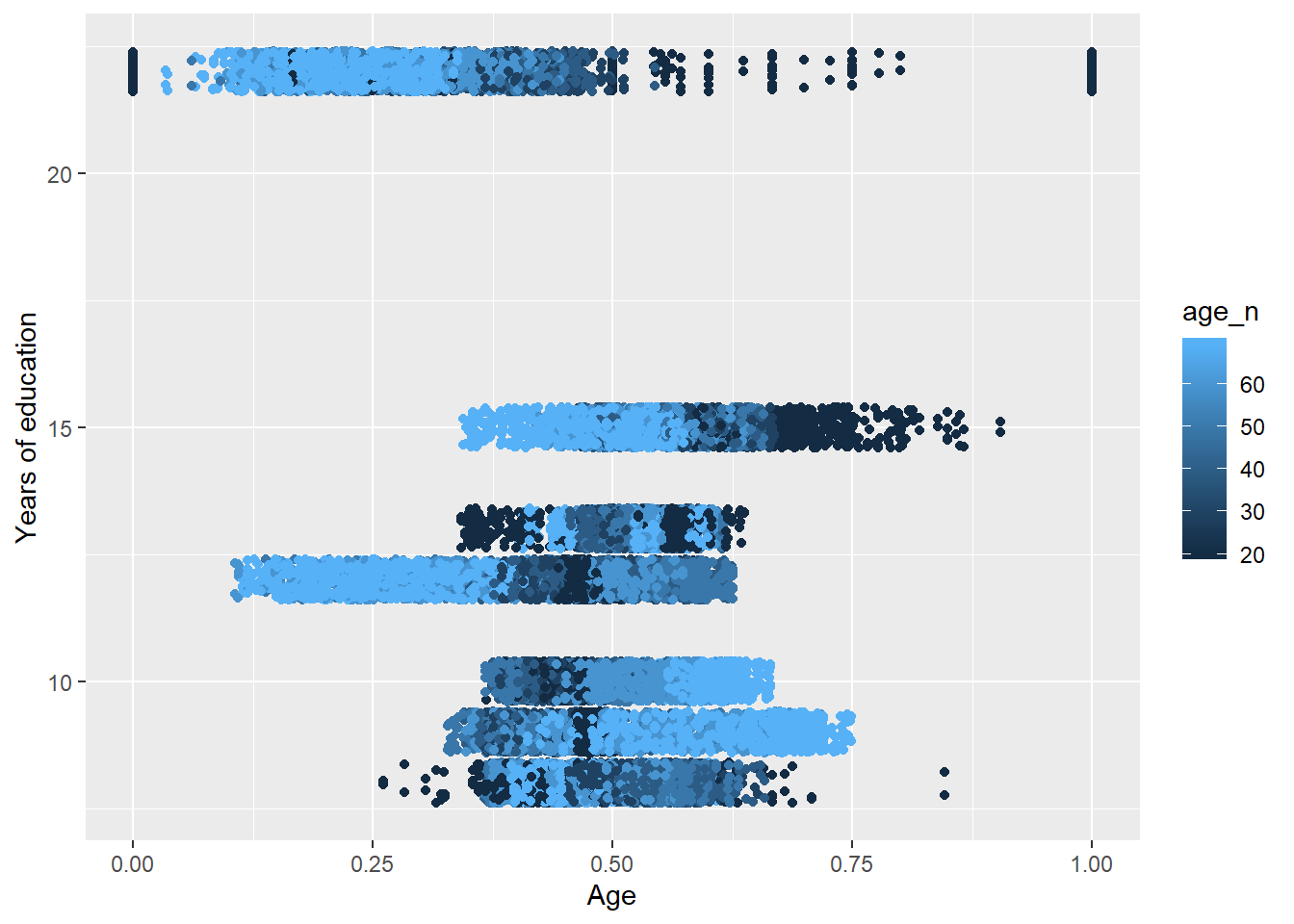
Figure 38: The significance of the interaction between per cent women and age on the level of education, Year 1985 - 2018
plot_model (model, type = "pred", terms = c("age_n", "sum_pop"))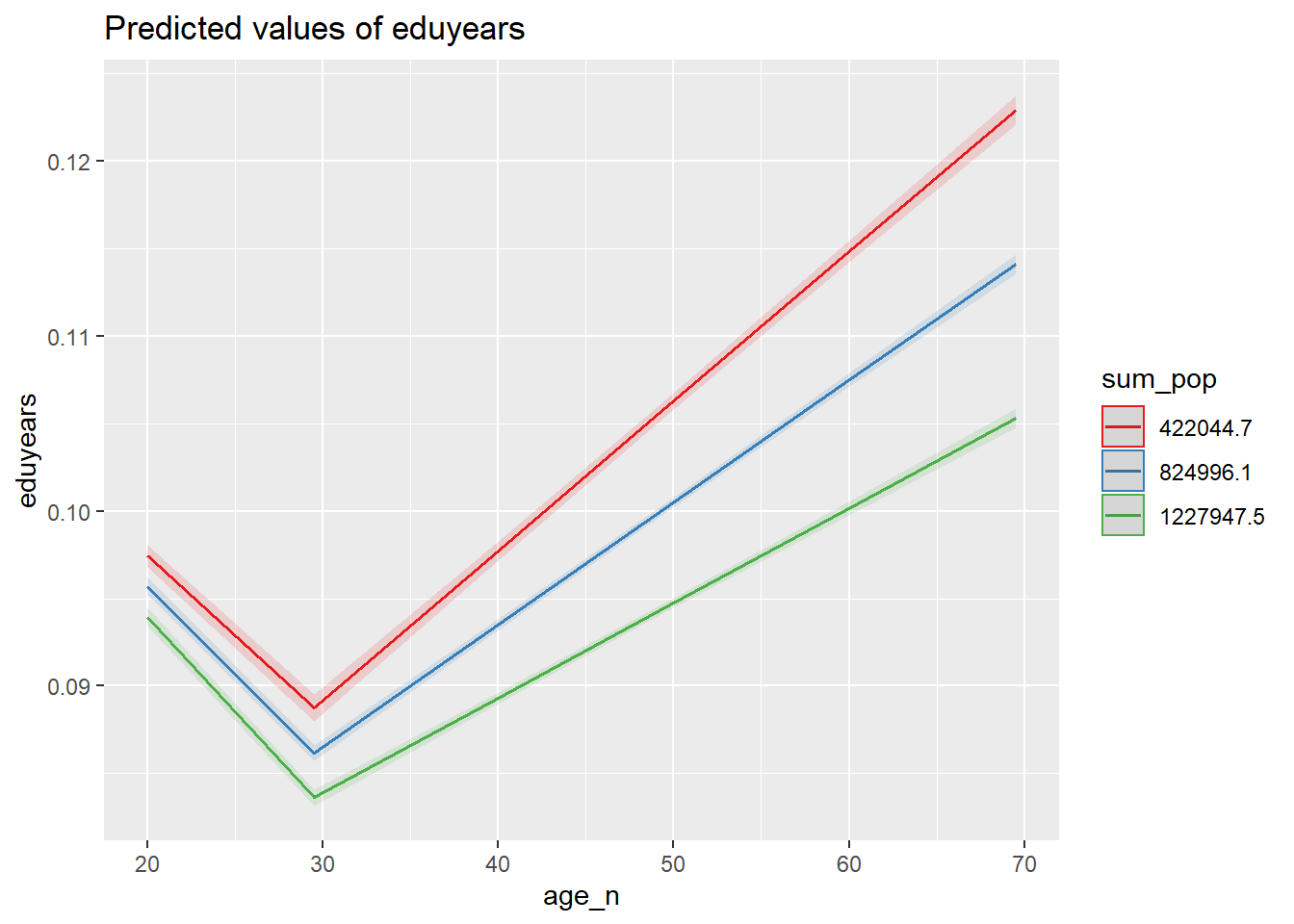
Figure 39: The significance of the interaction between the age and population in the region on the level of education, Year 1985 - 2018
plot_model (mmodel, type = "pred", terms = c("age_n", "sum_pop"))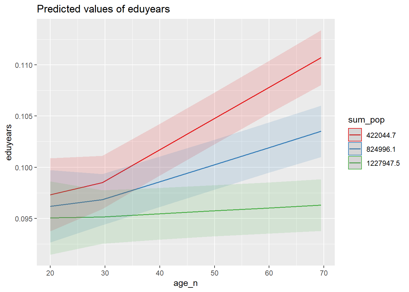
Figure 40: The significance of the interaction between the age and population in the region on the level of education, Year 1985 - 2018
tbnum %>%
  ggplot () +
    geom_jitter (mapping = aes(x = age_n, y = eduyears, colour = sum_pop)) +
  labs(
    x = "Age",
    y = "Years of education"
  )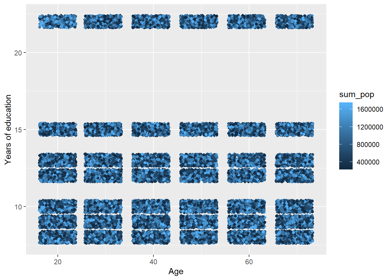
Figure 41: The significance of the interaction between the age and population in the region on the level of education, Year 1985 - 2018