For a couple of posts, I have analysed what predictors affect the education level in Sweden. In this post, I will return to analysing the salary of engineers and I will try to use my experiences from studying the education level.
Statistics Sweden use NUTS (Nomenclature des Unités Territoriales Statistiques), which is the EU’s hierarchical regional division, to specify the regions.
Please send suggestions for improvement of the analysis to ranalystatisticssweden@gmail.com.
First, define libraries and functions.
library (tidyverse)## -- Attaching packages -------------------------------------------------- tidyverse 1.3.0 --## v ggplot2 3.2.1 v purrr 0.3.3
## v tibble 2.1.3 v dplyr 0.8.3
## v tidyr 1.0.2 v stringr 1.4.0
## v readr 1.3.1 v forcats 0.4.0## -- Conflicts ----------------------------------------------------- tidyverse_conflicts() --
## x dplyr::filter() masks stats::filter()
## x dplyr::lag() masks stats::lag()library (broom)
library (car)## Loading required package: carData##
## Attaching package: 'car'## The following object is masked from 'package:dplyr':
##
## recode## The following object is masked from 'package:purrr':
##
## somelibrary (sjPlot)## Registered S3 methods overwritten by 'lme4':
## method from
## cooks.distance.influence.merMod car
## influence.merMod car
## dfbeta.influence.merMod car
## dfbetas.influence.merMod carlibrary (leaps)
library (MASS)##
## Attaching package: 'MASS'## The following object is masked from 'package:dplyr':
##
## selectlibrary (earth)## Warning: package 'earth' was built under R version 3.6.3## Loading required package: Formula## Loading required package: plotmo## Warning: package 'plotmo' was built under R version 3.6.3## Loading required package: plotrix## Loading required package: TeachingDemos## Warning: package 'TeachingDemos' was built under R version 3.6.3library (lspline)## Warning: package 'lspline' was built under R version 3.6.3library (boot)##
## Attaching package: 'boot'## The following object is masked from 'package:car':
##
## logitlibrary (faraway)##
## Attaching package: 'faraway'## The following objects are masked from 'package:boot':
##
## logit, melanoma## The following objects are masked from 'package:car':
##
## logit, viflibrary (arm)## Warning: package 'arm' was built under R version 3.6.3## Loading required package: Matrix##
## Attaching package: 'Matrix'## The following objects are masked from 'package:tidyr':
##
## expand, pack, unpack## Loading required package: lme4##
## arm (Version 1.10-1, built: 2018-4-12)## Working directory is C:/R/rblog/content/post##
## Attaching package: 'arm'## The following objects are masked from 'package:faraway':
##
## fround, logit, pfround## The following object is masked from 'package:boot':
##
## logit## The following object is masked from 'package:plotrix':
##
## rescale## The following object is masked from 'package:car':
##
## logitlibrary (caret) ## Warning: package 'caret' was built under R version 3.6.3## Loading required package: lattice##
## Attaching package: 'lattice'## The following object is masked from 'package:faraway':
##
## melanoma## The following object is masked from 'package:boot':
##
## melanoma##
## Attaching package: 'caret'## The following object is masked from 'package:purrr':
##
## liftlibrary (recipes) ## Warning: package 'recipes' was built under R version 3.6.3##
## Attaching package: 'recipes'## The following object is masked from 'package:stringr':
##
## fixed## The following object is masked from 'package:stats':
##
## steplibrary (vip) ## Warning: package 'vip' was built under R version 3.6.3##
## Attaching package: 'vip'## The following object is masked from 'package:utils':
##
## vilibrary (pdp) ## Warning: package 'pdp' was built under R version 3.6.3##
## Attaching package: 'pdp'## The following object is masked from 'package:faraway':
##
## pima## The following object is masked from 'package:purrr':
##
## partiallibrary (PerformanceAnalytics)## Warning: package 'PerformanceAnalytics' was built under R version 3.6.3## Loading required package: xts## Loading required package: zoo##
## Attaching package: 'zoo'## The following objects are masked from 'package:base':
##
## as.Date, as.Date.numeric##
## Attaching package: 'xts'## The following objects are masked from 'package:dplyr':
##
## first, last##
## Attaching package: 'PerformanceAnalytics'## The following object is masked from 'package:graphics':
##
## legendlibrary (ggpubr)## Warning: package 'ggpubr' was built under R version 3.6.3## Loading required package: magrittr##
## Attaching package: 'magrittr'## The following object is masked from 'package:purrr':
##
## set_names## The following object is masked from 'package:tidyr':
##
## extractlibrary (glmnet)## Warning: package 'glmnet' was built under R version 3.6.3## Loaded glmnet 3.0-2library (rpart) ##
## Attaching package: 'rpart'## The following object is masked from 'package:faraway':
##
## solderlibrary (ipred) ## Warning: package 'ipred' was built under R version 3.6.3readfile <- function (file1){read_csv (file1, col_types = cols(), locale = readr::locale (encoding = "latin1"), na = c("..", "NA")) %>%
gather (starts_with("19"), starts_with("20"), key = "year", value = groupsize) %>%
drop_na() %>%
mutate (year_n = parse_number (year))
}
perc_women <- function(x){
ifelse (length(x) == 2, x[2] / (x[1] + x[2]), NA)
}
nuts <- read.csv("nuts.csv") %>%
mutate(NUTS2_sh = substr(NUTS2, 3, 4))
nuts %>%
distinct (NUTS2_en) %>%
knitr::kable(
booktabs = TRUE,
caption = 'Nomenclature des Unités Territoriales Statistiques (NUTS)')| NUTS2_en |
|---|
| SE11 Stockholm |
| SE12 East-Central Sweden |
| SE21 Småland and islands |
| SE22 South Sweden |
| SE23 West Sweden |
| SE31 North-Central Sweden |
| SE32 Central Norrland |
| SE33 Upper Norrland |
bs <- function(formula, data, indices) {
  d <- data[indices,] # allows boot to select sample
  fit <- lm(formula, weights = tbnum_weights, data=d)
  return(coef(fit))
}
The data tables are downloaded from Statistics Sweden. They are saved as a comma-delimited file without heading, UF0506A1.csv, http://www.statistikdatabasen.scb.se/pxweb/en/ssd/.
The tables:
UF0506A1_1.csv: Population 16-74 years of age by region, highest level of education, age and sex. Year 1985 - 2018 NUTS 2 level 2008- 10 year intervals (16-74)
000000CG_1: Average basic salary, monthly salary and women´s salary as a percentage of men´s salary by region, sector, occupational group (SSYK 2012) and sex. Year 2014 - 2018 Monthly salary All sectors.
000000CD_1.csv: Average basic salary, monthly salary and women´s salary as a percentage of men´s salary by region, sector, occupational group (SSYK 2012) and sex. Year 2014 - 2018 Number of employees All sectors-
The data is aggregated, the size of each group is in the column groupsize.
I have also included some calculated predictors from the original data.
perc_women: The percentage of women within each group defined by edulevel, region and year
perc_women_region: The percentage of women within each group defined by year and region
regioneduyears: The average number of education years per capita within each group defined by sex, year and region
eduquotient: The quotient between regioneduyears for men and women
salaryquotient: The quotient between salary for men and women within each group defined by year and region
perc_women_eng_region: The percentage of women who are engineers within each group defined by year and region
numedulevel <- read.csv("edulevel_1.csv")

numedulevel[, 2] <- data.frame(c(8, 9, 10, 12, 13, 15, 22, NA))

tb <- readfile("000000CG_1.csv")
tb <- readfile("000000CD_1.csv") %>%
  left_join(tb, by = c("region", "year", "sex", "sector","occuptional  (SSYK 2012)")) %>%
  filter(`occuptional  (SSYK 2012)` == "214 Engineering professionals")

tb <- readfile("UF0506A1_1.csv") %>%
  right_join(tb, by = c("region", "year", "sex")) %>%
  right_join(numedulevel, by = c("level of education" = "level.of.education")) %>%
  filter(!is.na(eduyears)) %>%
  mutate(edulevel = `level of education`) %>%
  group_by(edulevel, region, year, sex) %>%
  mutate(groupsize_all_ages = sum(groupsize)) %>%
  group_by(edulevel, region, year) %>%
  mutate (perc_women = perc_women (groupsize_all_ages[1:2])) %>%
  group_by (sex, year, region) %>%
  mutate(regioneduyears = sum(groupsize * eduyears) / sum(groupsize)) %>%
  mutate(regiongroupsize = sum(groupsize)) %>%
  mutate(suming = groupsize.x) %>%
  group_by(region, year) %>%
  mutate (sum_pop = sum(groupsize)) %>%
  mutate (perc_women_region = perc_women (regiongroupsize[1:2])) %>%
  mutate (eduquotient = regioneduyears[2] / regioneduyears[1]) %>%
  mutate (salary = groupsize.y) %>%
  mutate (salaryquotient = salary[2] / salary[1]) %>%
  mutate (perc_women_eng_region = perc_women(suming[1:2])) %>%
  left_join(nuts %>% distinct (NUTS2_en, NUTS2_sh), by = c("region" = "NUTS2_en")) %>%
  drop_na()
## Warning: Column `level of education`/`level.of.education` joining character
## vector and factor, coercing into character vector## Warning: Column `region`/`NUTS2_en` joining character vector and factor,
## coercing into character vectorsummary(tb)## region age level of education sex
## Length:532 Length:532 Length:532 Length:532
## Class :character Class :character Class :character Class :character
## Mode :character Mode :character Mode :character Mode :character
##
##
##
## year groupsize year_n sector
## Length:532 Min. : 405 Min. :2014 Length:532
## Class :character 1st Qu.: 20996 1st Qu.:2015 Class :character
## Mode :character Median : 43656 Median :2016 Mode :character
## Mean : 64760 Mean :2016
## 3rd Qu.:102394 3rd Qu.:2017
## Max. :271889 Max. :2018
## occuptional (SSYK 2012) groupsize.x year_n.x groupsize.y
## Length:532 Min. : 340 Min. :2014 Min. :34700
## Class :character 1st Qu.: 1700 1st Qu.:2015 1st Qu.:40300
## Mode :character Median : 3000 Median :2016 Median :42000
## Mean : 5850 Mean :2016 Mean :42078
## 3rd Qu.: 7475 3rd Qu.:2017 3rd Qu.:43925
## Max. :21400 Max. :2018 Max. :49400
## year_n.y eduyears edulevel groupsize_all_ages
## Min. :2014 Min. : 8.00 Length:532 Min. : 405
## 1st Qu.:2015 1st Qu.: 9.00 Class :character 1st Qu.: 20996
## Median :2016 Median :12.00 Mode :character Median : 43656
## Mean :2016 Mean :12.71 Mean : 64760
## 3rd Qu.:2017 3rd Qu.:15.00 3rd Qu.:102394
## Max. :2018 Max. :22.00 Max. :271889
## perc_women regioneduyears regiongroupsize suming
## Min. :0.3575 Min. :11.18 Min. :128262 Min. : 340
## 1st Qu.:0.4338 1st Qu.:11.61 1st Qu.:288058 1st Qu.: 1700
## Median :0.4631 Median :11.74 Median :514608 Median : 3000
## Mean :0.4771 Mean :11.79 Mean :453318 Mean : 5850
## 3rd Qu.:0.5132 3rd Qu.:12.04 3rd Qu.:691870 3rd Qu.: 7475
## Max. :0.6423 Max. :12.55 Max. :827940 Max. :21400
## sum_pop perc_women_region eduquotient salary
## Min. : 262870 Min. :0.4831 Min. :1.019 Min. :34700
## 1st Qu.: 587142 1st Qu.:0.4882 1st Qu.:1.029 1st Qu.:40300
## Median :1029820 Median :0.4934 Median :1.034 Median :42000
## Mean : 906635 Mean :0.4923 Mean :1.034 Mean :42078
## 3rd Qu.:1395157 3rd Qu.:0.4970 3rd Qu.:1.041 3rd Qu.:43925
## Max. :1655215 Max. :0.5014 Max. :1.047 Max. :49400
## salaryquotient perc_women_eng_region NUTS2_sh
## Min. :0.8653 Min. :0.1566 Length:532
## 1st Qu.:0.9329 1st Qu.:0.1787 Class :character
## Median :0.9395 Median :0.2042 Mode :character
## Mean :0.9447 Mean :0.2039
## 3rd Qu.:0.9537 3rd Qu.:0.2216
## Max. :1.0446 Max. :0.2746Prepare the data using Tidyverse recipes package, i.e. centre, scale and make sure all predictors are numerical.
tbtemp <- ungroup(tb) %>% dplyr::select(region, salary, year_n, regiongroupsize, sex, regioneduyears, suming, perc_women_region, salaryquotient, eduquotient, perc_women_eng_region)

tb_outliers_info <- unique(tbtemp)

tb_unique <- unique(dplyr::select(tbtemp, -region))

tbnum_weights <- tb_unique$suming

blueprint <- recipe(salary ~ ., data = tb_unique) %>%
  step_nzv(all_nominal()) %>%
  step_integer(matches("Qual|Cond|QC|Qu")) %>%
  step_center(all_numeric(), -all_outcomes()) %>%
  step_scale(all_numeric(), -all_outcomes()) %>%
  step_dummy(all_nominal(), -all_outcomes(), one_hot = TRUE)

prepare <- prep(blueprint, training = tb_unique)

tbnum <- bake(prepare, new_data = tb_unique)
The correlation chart shows that many predictors are correlated with the response variable but also that many predictors are correlated between each other. The vif function also shows high multicollinearity. Some notable correlations are in a dedicated plot below.
chart.Correlation(tbnum, histogram = TRUE, pch = 19)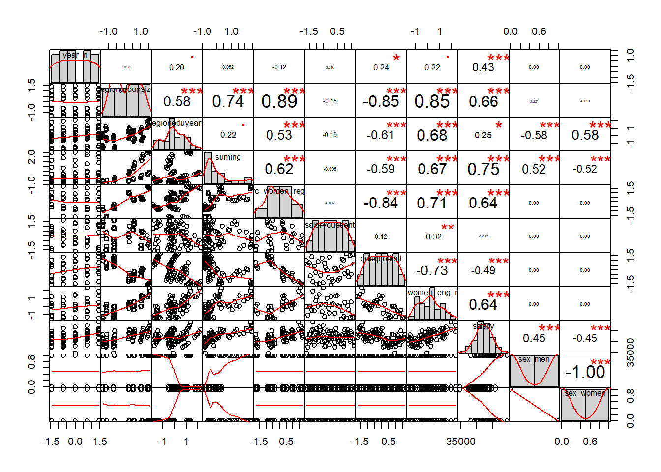
Figure 1: Correlation between response and predictors and between predictors, Year 2014 - 2018
vif(tbnum)## Warning in summary.lm(lm(object[, i] ~ object[, -i])): essentially perfect fit:
## summary may be unreliable
## Warning in summary.lm(lm(object[, i] ~ object[, -i])): essentially perfect fit:
## summary may be unreliable## year_n regiongroupsize regioneduyears
## 4.665634 21.810910 14.478685
## suming perc_women_region salaryquotient
## 8.688599 8.259497 1.382593
## eduquotient perc_women_eng_region salary
## 12.400845 8.141404 8.359112
## sex_men sex_women
## Inf Infp1 <- tb %>%
ggscatter(x = "regiongroupsize", y = "perc_women_region",
add = "reg.line", conf.int = TRUE,
cor.coef = TRUE, cor.method = "pearson")
p2 <- tb %>%
ggscatter(x = "regiongroupsize", y = "perc_women_eng_region",
add = "reg.line", conf.int = TRUE,
cor.coef = TRUE, cor.method = "pearson")
p3 <- tb %>%
ggscatter(x = "regiongroupsize", y = "eduquotient",
add = "reg.line", conf.int = TRUE,
cor.coef = TRUE, cor.method = "pearson")
p4 <- tb %>%
ggscatter(x = "perc_women_region", y = "eduquotient",
add = "reg.line", conf.int = TRUE,
cor.coef = TRUE, cor.method = "pearson")
gridExtra::grid.arrange(p1, p2, p3, p4, ncol = 2)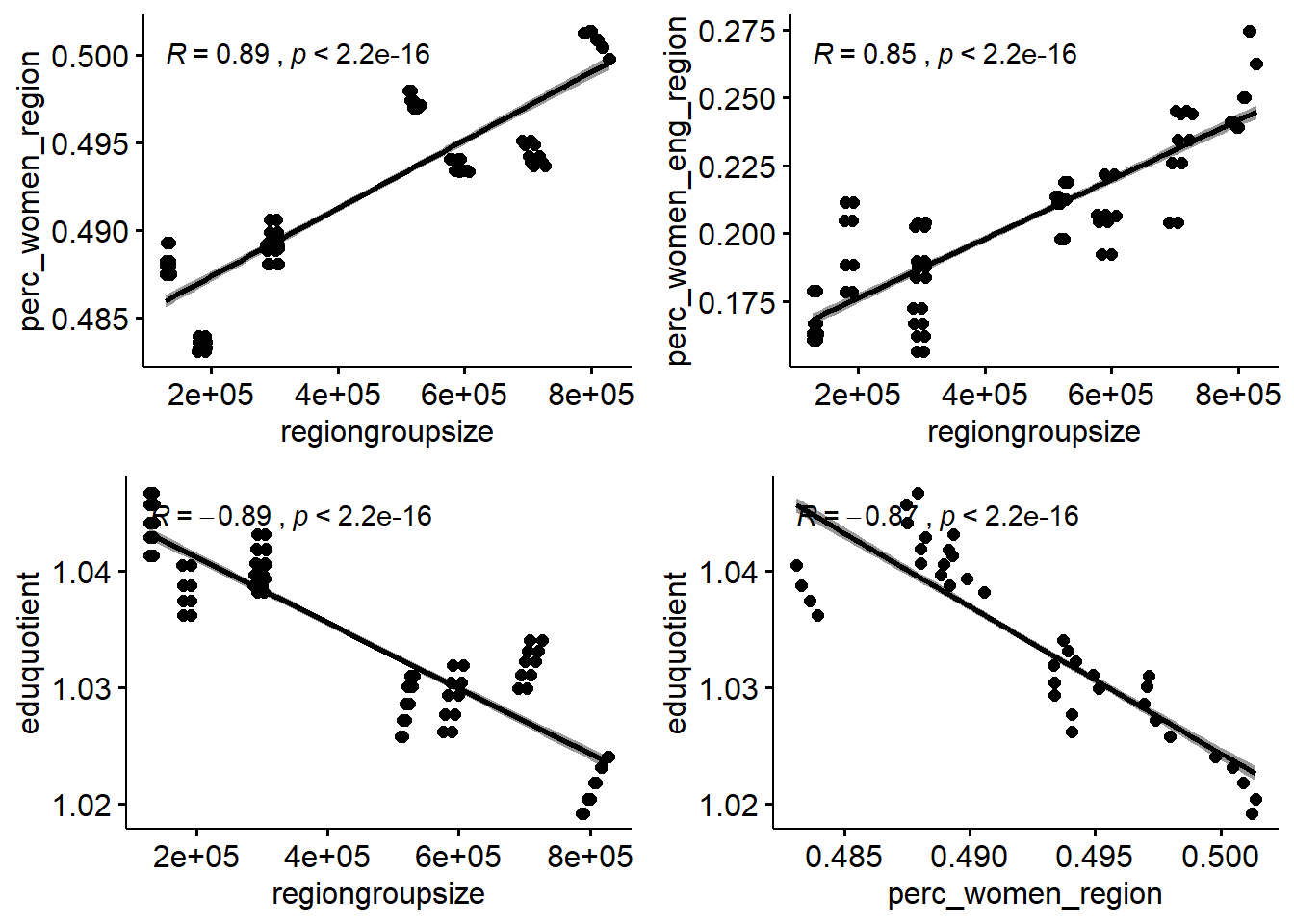
Figure 2: Correlation between response and predictors and between predictors, Year 2014 - 2018
The dataset only contains 76 rows. This together with multicollinearity limits the number of predictors to include in the regression. I would like to choose the predictors that best contains most information from the dataset with respect to the response.
I will use an elastic net to find the variable that contains the best signals for later use in the analysis. First I will search for the explanatory variables that best predict the response using no interactions. I will use 10-fold cross-validation with an elastic net. Elastic nets are linear and do not take into account the shape of the relations between the predictors. Alpha = 1 indicates a lasso regression.
X <- model.matrix(salary ~ ., tbnum)[, -1]

Y <- tbnum$salary

set.seed(123)  # for reproducibility
cv_glmnet <- train(
    x = X,
    y = Y,
    weights = tbnum_weights,
    method = "glmnet",
    preProc = c("zv", "center", "scale"),
    trControl = trainControl(method = "cv", number = 10),
    tuneLength = 20
)
## Warning in nominalTrainWorkflow(x = x, y = y, wts = weights, info = trainInfo, :
## There were missing values in resampled performance measures.vip(cv_glmnet, num_features = 20, geom = "point")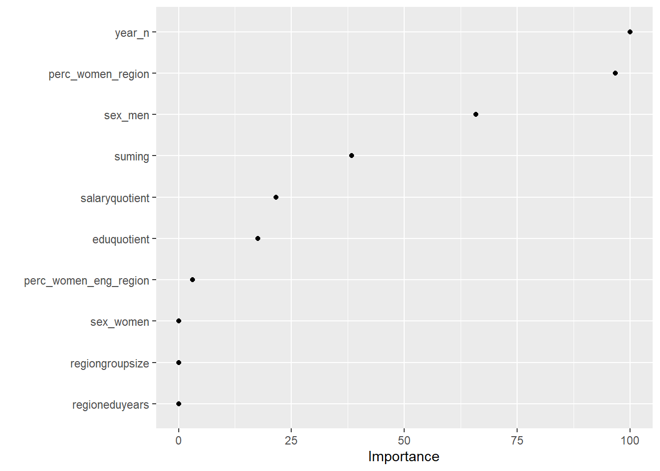
Figure 3: Elastic net search on the data using no interactions, Year 2014 - 2018
cv_glmnet$bestTune## alpha lambda
## 371 1 49.48132elastic_min <- glmnet(
x = X,
y = Y,
alpha = 1
)
plot(elastic_min, xvar = "lambda", main = "Elastic net penalty\n\n")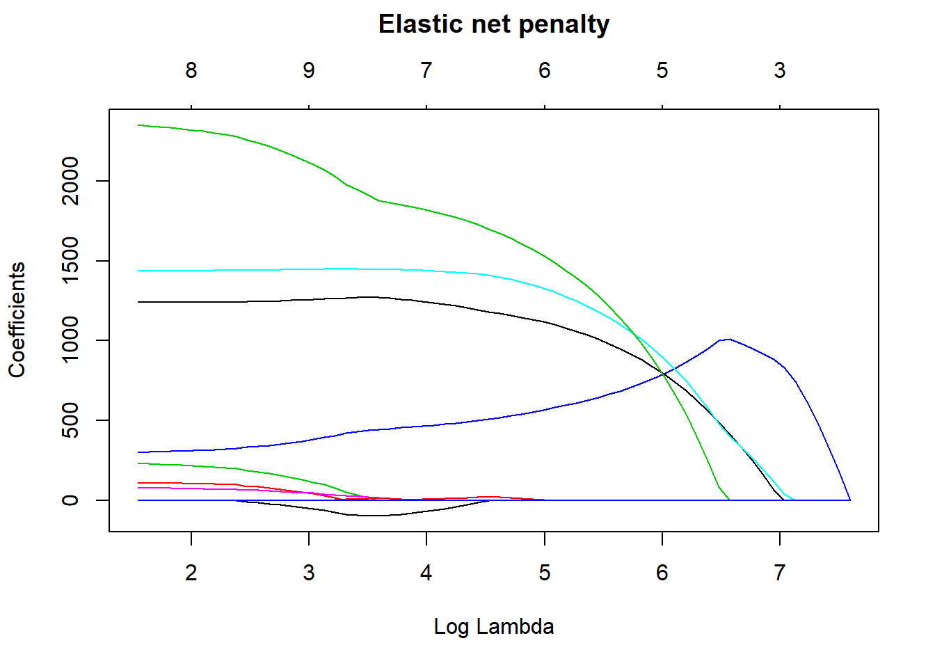
Figure 4: Elastic net search on the data using no interactions, Year 2014 - 2018
Next, I will use an elastic net to find the variable that contains the best signals including interactions.
temp <- dplyr::select(tbnum, -salary)

f <- as.formula( ~ .*.)
X <- model.matrix(f, temp)[, -1]

Y <- tbnum$salary

set.seed(123)  # for reproducibility
cv_glmnet <- train(
    x = X,
    y = Y,
    weights = tbnum_weights,
    method = "glmnet",
    metric = "Rsquared",
    maximize = TRUE,
    preProc = c("zv", "center", "scale"),
    trControl = trainControl(method = "cv", number = 10),
    tuneLength = 30
)
## Warning in nominalTrainWorkflow(x = x, y = y, wts = weights, info = trainInfo, :
## There were missing values in resampled performance measures.## Warning in train.default(x = X, y = Y, weights = tbnum_weights, method =
## "glmnet", : missing values found in aggregated resultsvip(cv_glmnet, num_features = 20, geom = "point")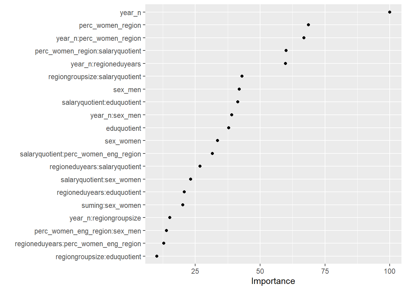
Figure 5: Elastic net search on the data including interactions, Year 2014 - 2018
cv_glmnet$bestTune## alpha lambda
## 758 0.8758621 4.280173elastic_min <- glmnet(
x = X,
y = Y,
alpha = 0.9
)
plot(elastic_min, xvar = "lambda", main = "Elastic net penalty\n\n")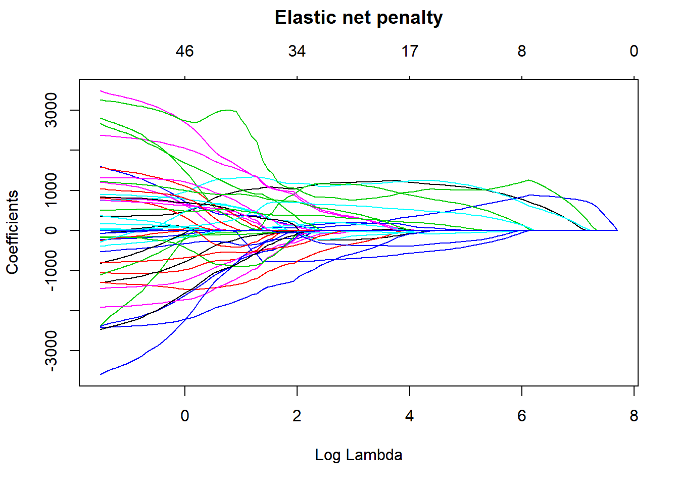
Figure 6: Elastic net search on the data including interactions, Year 2014 - 2018
I use MARS to fit the best signals using from the elastic net using no interactions. Four predictors minimise the AIC while still ensuring that the coefficients are valid, testing them with bootstrap.
temp <- dplyr::select(tbnum, c(salary, year_n, sex_men, perc_women_region, suming))

mmod_scaled <- earth(salary ~ ., weights = tbnum_weights, data = temp, nk = 9, degree = 1)

summary (mmod_scaled)
## Call: earth(formula=salary~., data=temp, weights=tbnum_weights, degree=1, nk=9)
##
## coefficients
## (Intercept) 40889.888
## sex_men 1684.691
## h(0-year_n) -884.328
## h(year_n-0) 1673.931
## h(0.311813-perc_women_region) -1249.276
## h(perc_women_region-0.311813) 1754.546
## h(suming- -0.549566) 553.529
##
## Selected 7 of 8 terms, and 4 of 4 predictors
## Termination condition: Reached nk 9
## Importance: suming, year_n, perc_women_region, sex_men
## Weights: 21400, 6800, 11500, 3000, 2400, 500, 7000, 1900, 16000, 4100, 3...
## Number of terms at each degree of interaction: 1 6 (additive model)
## GCV 3373591806 RSS 176181393125 GRSq 0.9000639 RSq 0.9294851plot (mmod_scaled)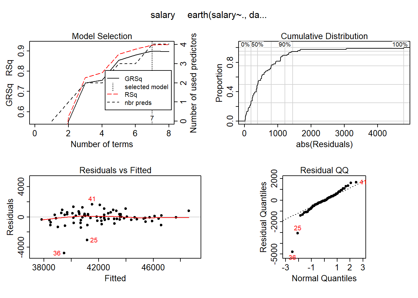
Figure 7: Hockey-stick functions fit with MARS for the predictors using no interactions, Year 2014 - 2018
plotmo (mmod_scaled)## plotmo grid: year_n sex_men perc_women_region suming
## 0 0.5 0.2069953 -0.4539968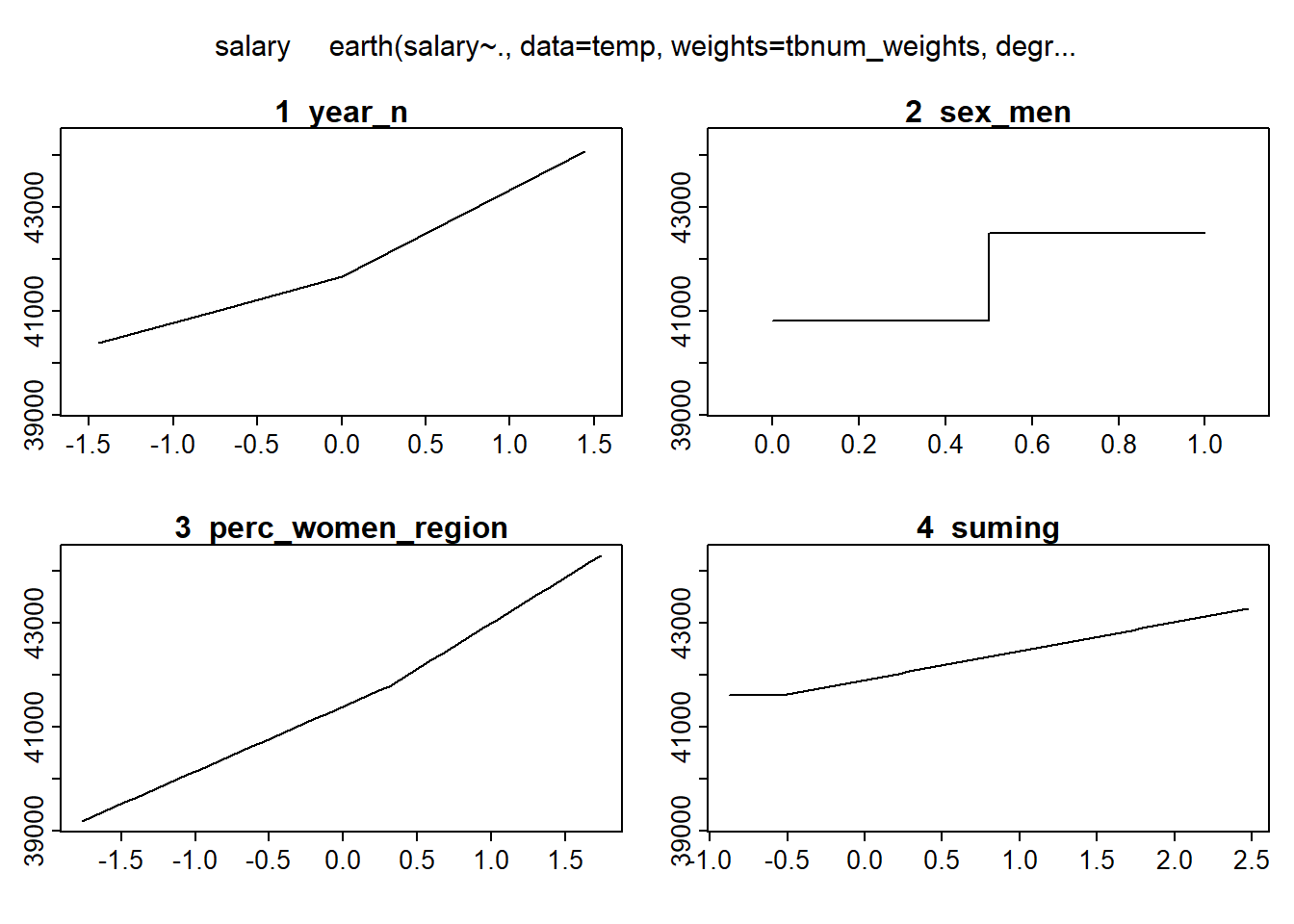
Figure 8: Hockey-stick functions fit with MARS for the predictors using no interactions, Year 2014 - 2018
model_mmod_scale <- lm (salary ~
  sex_men +
  lspline(year_n, c(0)) +
  lspline(perc_women_region, c(0.311813)) +
  lspline(suming, c(-0.549566)),
  weights = tbnum_weights,
  data = tbnum)

b <- regsubsets(salary ~ sex_men + lspline(year_n, c(0)) + lspline(perc_women_region, c(0.311813)) + lspline(suming, c(-0.549566)) + lspline(suming, c(-1.22297)), data = tbnum, weights = tbnum_weights, nvmax = 12)
## Warning in leaps.setup(x, y, wt = wt, nbest = nbest, nvmax = nvmax, force.in =
## force.in, : 2 linear dependencies found## Warning in leaps.setup(x, y, wt = wt, nbest = nbest, nvmax = nvmax, force.in =
## force.in, : nvmax reduced to 7rs <- summary(b)
AIC <- 50 * log (rs$rss / 50) + (2:8) * 2
which.min (AIC)## [1] 6names (rs$which[6,])[rs$which[6,]]## [1] "(Intercept)"
## [2] "sex_men"
## [3] "lspline(year_n, c(0))1"
## [4] "lspline(year_n, c(0))2"
## [5] "lspline(perc_women_region, c(0.311813))1"
## [6] "lspline(perc_women_region, c(0.311813))2"
## [7] "lspline(suming, c(-1.22297))2"model_mmod_scale <- lm (salary ~
sex_men +
lspline(year_n, c(0)) +
lspline(perc_women_region, c(0.311813)) +
lspline(suming, c(-0.549566)),
weights = tbnum_weights,
data = tbnum)
summary (model_mmod_scale)$adj.r.squared## [1] 0.9244956AIC(model_mmod_scale)## [1] 1258.423set.seed(123)
results <- boot(data = tbnum, statistic = bs,
R = 1000, formula = as.formula(model_mmod_scale))
#conf = coefficient not passing through zero
summary (model_mmod_scale) %>% tidy() %>%
mutate(bootest = tidy(results)$statistic,
bootbias = tidy(results)$bias,
booterr = tidy(results)$std.error,
conf = !((tidy(confint(results))$X2.5.. < 0) & (tidy(confint(results))$X97.5.. > 0)))## Warning in norm.inter(t, adj.alpha): extreme order statistics used as endpoints## Warning: 'tidy.matrix' is deprecated.
## See help("Deprecated")## Warning in norm.inter(t, adj.alpha): extreme order statistics used as endpoints## Warning: 'tidy.matrix' is deprecated.
## See help("Deprecated")## # A tibble: 8 x 9
## term estimate std.error statistic p.value bootest bootbias booterr conf
## <chr> <dbl> <dbl> <dbl> <dbl> <dbl> <dbl> <dbl> <lgl>
## 1 (Interce~ 42276. 1260. 33.6 4.85e-44 42276. -105. 1344. TRUE
## 2 sex_men 1502. 299. 5.02 4.02e- 6 1502. 27.6 428. TRUE
## 3 lspline(~ 868. 164. 5.31 1.32e- 6 868. -78.3 354. TRUE
## 4 lspline(~ 1656. 159. 10.4 9.25e-16 1656. 58.4 352. TRUE
## 5 lspline(~ 1049. 274. 3.82 2.88e- 4 1049. 146. 327. TRUE
## 6 lspline(~ 1719. 161. 10.7 3.31e-16 1719. -155. 265. TRUE
## 7 lspline(~ 2979. 2084. 1.43 1.57e- 1 2979. -264. 2216. FALSE
## 8 lspline(~ 603. 129. 4.66 1.52e- 5 603. -42.0 204. TRUEplot(results, index=1) # intercept 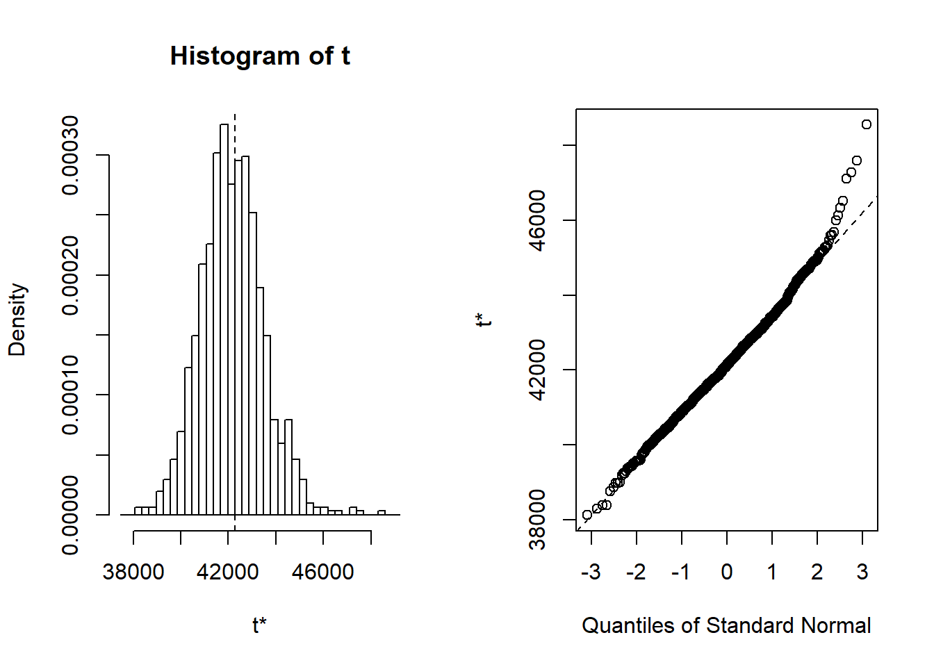
Figure 9: Hockey-stick functions fit with MARS for the predictors using no interactions, Year 2014 - 2018
I will include the interaction between sex_men and salaryquotient. If I include more terms from MARS I judge that the predictions are getting unstable testing with bootstrap.
# The three best candidates from the elastic net search
model_mmod_scale <- lm (salary ~
year_n +
perc_women_region +
year_n:perc_women_region,
weights = tbnum_weights,
data = tbnum)
summary (model_mmod_scale)##
## Call:
## lm(formula = salary ~ year_n + perc_women_region + year_n:perc_women_region,
## data = tbnum, weights = tbnum_weights)
##
## Weighted Residuals:
## Min 1Q Median 3Q Max
## -210878 -73763 -29626 45157 267181
##
## Coefficients:
## Estimate Std. Error t value Pr(>|t|)
## (Intercept) 42830.76 200.55 213.569 < 2e-16 ***
## year_n 1362.05 205.00 6.644 4.97e-09 ***
## perc_women_region 1953.39 187.13 10.439 4.66e-16 ***
## year_n:perc_women_region -32.32 194.19 -0.166 0.868
## ---
## Signif. codes: 0 '***' 0.001 '**' 0.01 '*' 0.05 '.' 0.1 ' ' 1
##
## Residual standard error: 102900 on 72 degrees of freedom
## Multiple R-squared: 0.6949, Adjusted R-squared: 0.6822
## F-statistic: 54.65 on 3 and 72 DF, p-value: < 2.2e-16set.seed(123)
results <- boot(data = tbnum, statistic = bs,
R = 1000, formula = as.formula(model_mmod_scale))
summary (model_mmod_scale) %>% tidy() %>%
mutate(bootest = tidy(results)$statistic,
bootbias = tidy(results)$bias,
booterr = tidy(results)$std.error,
conf = !((tidy(confint(results))$X2.5.. < 0) & (tidy(confint(results))$X97.5.. > 0)))## Warning in confint.boot(results): BCa method fails for this problem. Using
## 'perc' instead## Warning: 'tidy.matrix' is deprecated.
## See help("Deprecated")## Warning in confint.boot(results): BCa method fails for this problem. Using
## 'perc' instead## Warning: 'tidy.matrix' is deprecated.
## See help("Deprecated")## # A tibble: 4 x 9
## term estimate std.error statistic p.value bootest bootbias booterr conf
## <chr> <dbl> <dbl> <dbl> <dbl> <dbl> <dbl> <dbl> <lgl>
## 1 (Interc~ 42831. 201. 214. 1.22e-102 42831. -776. 254. TRUE
## 2 year_n 1362. 205. 6.64 4.97e- 9 1362. 10.8 253. TRUE
## 3 perc_wo~ 1953. 187. 10.4 4.66e- 16 1953. -94.0 273. TRUE
## 4 year_n:~ -32.3 194. -0.166 8.68e- 1 -32.3 -73.3 291. FALSEtemp <- dplyr::select(tbnum, c(salary, year_n, sex_men, perc_women_region, suming, salaryquotient, regioneduyears))
# A test with MARS and interactions
mmod_scaled <- earth(salary ~ ., weights = tbnum_weights, data = temp, nk = 11, degree = 2)
summary (mmod_scaled)## Call: earth(formula=salary~., data=temp, weights=tbnum_weights, degree=2,
## nk=11)
##
## coefficients
## (Intercept) 41145.980
## sex_men 1911.153
## h(0-year_n) -959.068
## h(year_n-0) 1703.923
## h(0.311813-perc_women_region) -1598.885
## h(perc_women_region-0.311813) 1546.770
## h(suming- -0.549566) 377.482
## sex_men * salaryquotient -526.973
##
## Selected 8 of 9 terms, and 5 of 6 predictors
## Termination condition: Reached nk 11
## Importance: year_n, suming, perc_women_region, sex_men, salaryquotient, ...
## Weights: 21400, 6800, 11500, 3000, 2400, 500, 7000, 1900, 16000, 4100, 3...
## Number of terms at each degree of interaction: 1 6 1
## GCV 2668331064 RSS 116081178669 GRSq 0.9209559 RSq 0.9535396mmod_scaled <- earth(salary ~ ., weights = tbnum_weights, data = temp, nk = 13, degree = 2)
summary (mmod_scaled)## Call: earth(formula=salary~., data=temp, weights=tbnum_weights, degree=2,
## nk=13)
##
## coefficients
## (Intercept) 41200.129
## sex_men 1935.664
## h(0-year_n) -867.152
## h(year_n-0) 1727.342
## h(0.311813-perc_women_region) -1532.402
## h(perc_women_region-0.311813) 1450.579
## h(suming- -0.549566) 353.205
## h(-1.22297-salaryquotient) -3067.317
## sex_men * salaryquotient -647.409
##
## Selected 9 of 11 terms, and 5 of 6 predictors
## Termination condition: Reached nk 13
## Importance: year_n, suming, perc_women_region, sex_men, salaryquotient, ...
## Weights: 21400, 6800, 11500, 3000, 2400, 500, 7000, 1900, 16000, 4100, 3...
## Number of terms at each degree of interaction: 1 7 1
## GCV 2629100288 RSS 104645110144 GRSq 0.922118 RSq 0.9581168plot (mmod_scaled)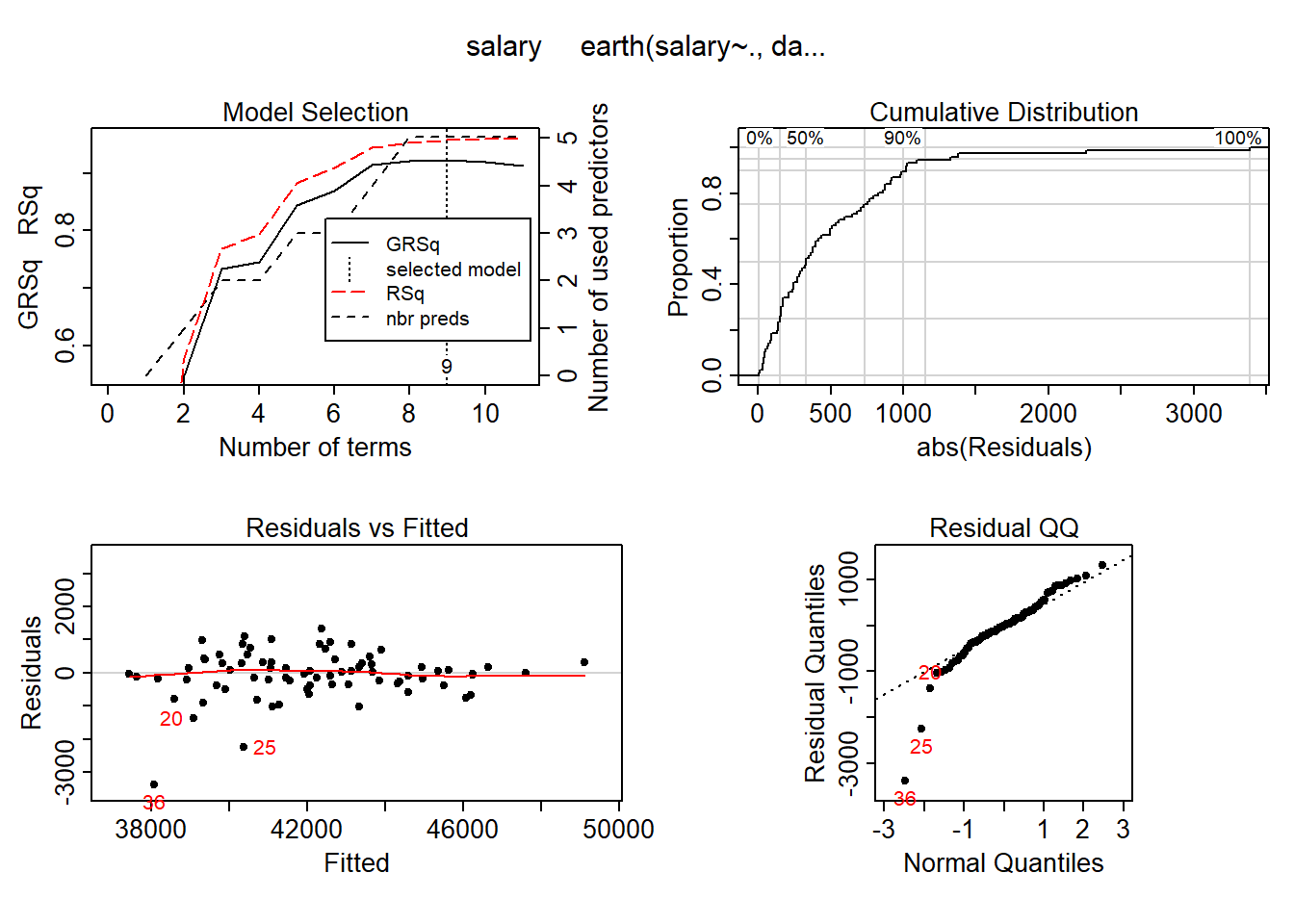
Figure 10: Hockey-stick functions fit with MARS for the predictors including interactions, Year 2014 - 2018
plotmo (mmod_scaled)## plotmo grid: year_n sex_men perc_women_region suming salaryquotient
## 0 0.5 0.2069953 -0.4539968 0
## regioneduyears
## -0.1394781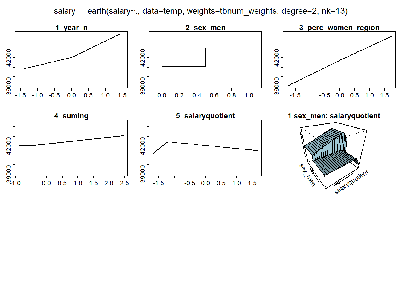
Figure 11: Hockey-stick functions fit with MARS for the predictors including interactions, Year 2014 - 2018
model_mmod_scale <- lm (salary ~
sex_men +
lspline(year_n, c(0)) +
lspline(perc_women_region, c(0.311813)) +
lspline(suming, c(-0.549566)) +
lspline(salaryquotient, c(-1.22297)) +
sex_men:salaryquotient,
weights = tbnum_weights,
data = tbnum)
summary (model_mmod_scale)##
## Call:
## lm(formula = salary ~ sex_men + lspline(year_n, c(0)) + lspline(perc_women_region,
## c(0.311813)) + lspline(suming, c(-0.549566)) + lspline(salaryquotient,
## c(-1.22297)) + sex_men:salaryquotient, data = tbnum, weights = tbnum_weights)
##
## Weighted Residuals:
## Min 1Q Median 3Q Max
## -159343 -17893 2866 18128 79279
##
## Coefficients:
## Estimate Std. Error t value Pr(>|t|)
## (Intercept) 44723.0 1743.3 25.655 < 2e-16
## sex_men 1772.4 238.2 7.440 2.88e-10
## lspline(year_n, c(0))1 868.1 131.4 6.606 8.56e-09
## lspline(year_n, c(0))2 1710.1 122.9 13.910 < 2e-16
## lspline(perc_women_region, c(0.311813))1 1382.3 225.1 6.142 5.51e-08
## lspline(perc_women_region, c(0.311813))2 1518.7 139.2 10.911 2.48e-16
## lspline(suming, c(-0.549566))1 1786.4 1624.5 1.100 0.275534
## lspline(suming, c(-0.549566))2 395.8 105.3 3.758 0.000369
## lspline(salaryquotient, c(-1.22297))1 2705.7 1126.2 2.403 0.019147
## lspline(salaryquotient, c(-1.22297))2 295.7 151.4 1.953 0.055071
## sex_men:salaryquotient -884.9 158.6 -5.578 5.07e-07
##
## (Intercept) ***
## sex_men ***
## lspline(year_n, c(0))1 ***
## lspline(year_n, c(0))2 ***
## lspline(perc_women_region, c(0.311813))1 ***
## lspline(perc_women_region, c(0.311813))2 ***
## lspline(suming, c(-0.549566))1
## lspline(suming, c(-0.549566))2 ***
## lspline(salaryquotient, c(-1.22297))1 *
## lspline(salaryquotient, c(-1.22297))2 .
## sex_men:salaryquotient ***
## ---
## Signif. codes: 0 '***' 0.001 '**' 0.01 '*' 0.05 '.' 0.1 ' ' 1
##
## Residual standard error: 38700 on 65 degrees of freedom
## Multiple R-squared: 0.961, Adjusted R-squared: 0.955
## F-statistic: 160.3 on 10 and 65 DF, p-value: < 2.2e-16set.seed(123)
results <- boot(data = tbnum, statistic = bs,
R = 1000, formula = as.formula(model_mmod_scale))
summary (model_mmod_scale) %>% tidy() %>%
mutate(bootest = tidy(results)$statistic,
bootbias = tidy(results)$bias,
booterr = tidy(results)$std.error,
conf = !((tidy(confint(results))$X2.5.. < 0) & (tidy(confint(results))$X97.5.. > 0)))## Warning: 'tidy.matrix' is deprecated.
## See help("Deprecated")
## Warning: 'tidy.matrix' is deprecated.
## See help("Deprecated")
## # A tibble: 11 x 9
## term estimate std.error statistic p.value bootest bootbias booterr conf
## <chr> <dbl> <dbl> <dbl> <dbl> <dbl> <dbl> <dbl> <lgl>
## 1 (Interc~ 44723. 1743. 25.7 1.02e-35 44723. 1007. 3439. TRUE
## 2 sex_men 1772. 238. 7.44 2.88e-10 1772. -3.65 339. TRUE
## 3 lspline~ 868. 131. 6.61 8.56e- 9 868. -88.4 299. TRUE
## 4 lspline~ 1710. 123. 13.9 3.71e-21 1710. -11.6 250. TRUE
## 5 lspline~ 1382. 225. 6.14 5.51e- 8 1382. -104. 308. TRUE
## 6 lspline~ 1519. 139. 10.9 2.48e-16 1519. -51.2 248. TRUE
## 7 lspline~ 1786. 1625. 1.10 2.76e- 1 1786. 80.7 1608. FALSE
## 8 lspline~ 396. 105. 3.76 3.69e- 4 396. 47.0 171. FALSE
## 9 lspline~ 2706. 1126. 2.40 1.91e- 2 2706. 904. 2568. FALSE
## 10 lspline~ 296. 151. 1.95 5.51e- 2 296. 77.6 196. FALSE
## 11 sex_men~ -885. 159. -5.58 5.07e- 7 -885. -153. 264. TRUEI will also use 10-fold cross-validation fit with decision trees and bagging on the data.
set.seed(123)
tbnum_bag <- train(
  salary ~ .,
  data = tbnum,
  method = "treebag",
  weights = tbnum_weights,
  trControl = trainControl(method = "cv", number = 10),
  nbagg = 200,
  control = rpart.control(minsplit = 2, cp = 0)
)

vip::vip(tbnum_bag, num_features = 20, bar = FALSE)
## Warning in vip.default(tbnum_bag, num_features = 20, bar = FALSE): The `bar`
## argument has been deprecated in favor of the new `geom` argument. It will be
## removed in version 0.3.0.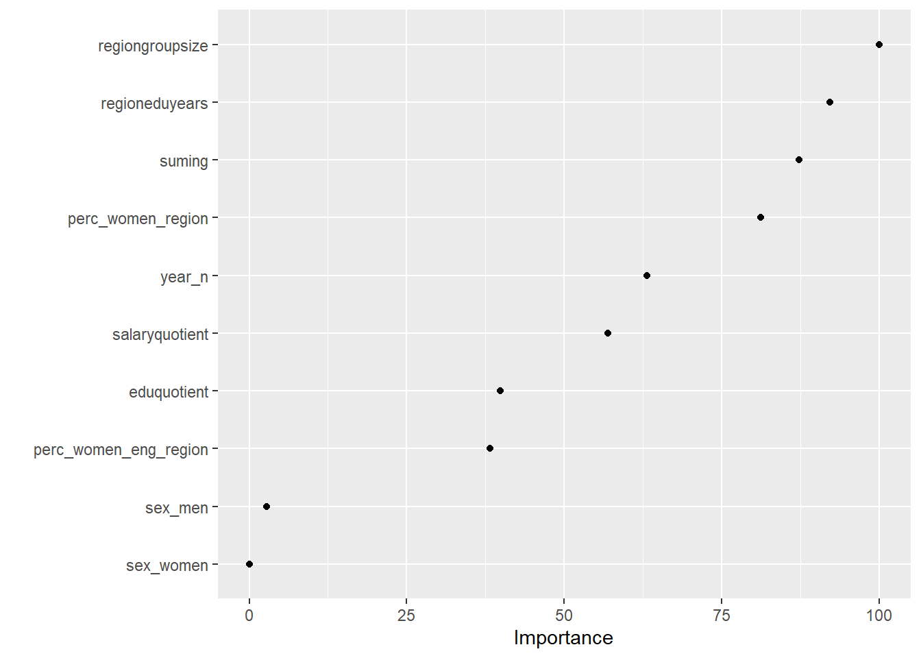
Figure 12: Data fit with decision tree bag, Year 2014 - 2018
Perform diagnostics on the final model.
model <- lm (salary ~
  sex_men +
  lspline(year_n, c(0)) +
  lspline(perc_women_region, c(0.311813)) +
  lspline(suming, c(-0.549566)) +
  sex_men:salaryquotient,
  weights = tbnum_weights,
  data = tbnum)

summary (model)
##
## Call:
## lm(formula = salary ~ sex_men + lspline(year_n, c(0)) + lspline(perc_women_region,
## c(0.311813)) + lspline(suming, c(-0.549566)) + sex_men:salaryquotient,
## data = tbnum, weights = tbnum_weights)
##
## Weighted Residuals:
## Min 1Q Median 3Q Max
## -158211 -13213 -2260 20760 84251
##
## Coefficients:
## Estimate Std. Error t value Pr(>|t|)
## (Intercept) 41612.74 1045.30 39.809 < 2e-16
## sex_men 1806.47 252.49 7.155 8.00e-10
## lspline(year_n, c(0))1 948.66 135.66 6.993 1.56e-09
## lspline(year_n, c(0))2 1693.55 131.00 12.928 < 2e-16
## lspline(perc_women_region, c(0.311813))1 1481.96 238.41 6.216 3.72e-08
## lspline(perc_women_region, c(0.311813))2 1531.75 136.49 11.222 < 2e-16
## lspline(suming, c(-0.549566))1 1625.10 1734.28 0.937 0.35210
## lspline(suming, c(-0.549566))2 408.52 112.02 3.647 0.00052
## sex_men:salaryquotient -515.55 89.72 -5.746 2.44e-07
##
## (Intercept) ***
## sex_men ***
## lspline(year_n, c(0))1 ***
## lspline(year_n, c(0))2 ***
## lspline(perc_women_region, c(0.311813))1 ***
## lspline(perc_women_region, c(0.311813))2 ***
## lspline(suming, c(-0.549566))1
## lspline(suming, c(-0.549566))2 ***
## sex_men:salaryquotient ***
## ---
## Signif. codes: 0 '***' 0.001 '**' 0.01 '*' 0.05 '.' 0.1 ' ' 1
##
## Residual standard error: 41350 on 67 degrees of freedom
## Multiple R-squared: 0.9541, Adjusted R-squared: 0.9487
## F-statistic: 174.2 on 8 and 67 DF, p-value: < 2.2e-16anova (model)## Analysis of Variance Table
##
## Response: salary
## Df Sum Sq Mean Sq F value
## sex_men 1 4.1914e+11 4.1914e+11 245.090
## lspline(year_n, c(0)) 2 6.3234e+11 3.1617e+11 184.879
## lspline(perc_women_region, c(0.311813)) 2 1.2213e+12 6.1063e+11 357.064
## lspline(suming, c(-0.549566)) 2 5.4719e+10 2.7360e+10 15.998
## sex_men:salaryquotient 1 5.6461e+10 5.6461e+10 33.015
## Residuals 67 1.1458e+11 1.7101e+09
## Pr(>F)
## sex_men < 2.2e-16 ***
## lspline(year_n, c(0)) < 2.2e-16 ***
## lspline(perc_women_region, c(0.311813)) < 2.2e-16 ***
## lspline(suming, c(-0.549566)) 2.090e-06 ***
## sex_men:salaryquotient 2.439e-07 ***
## Residuals
## ---
## Signif. codes: 0 '***' 0.001 '**' 0.01 '*' 0.05 '.' 0.1 ' ' 1plot (model)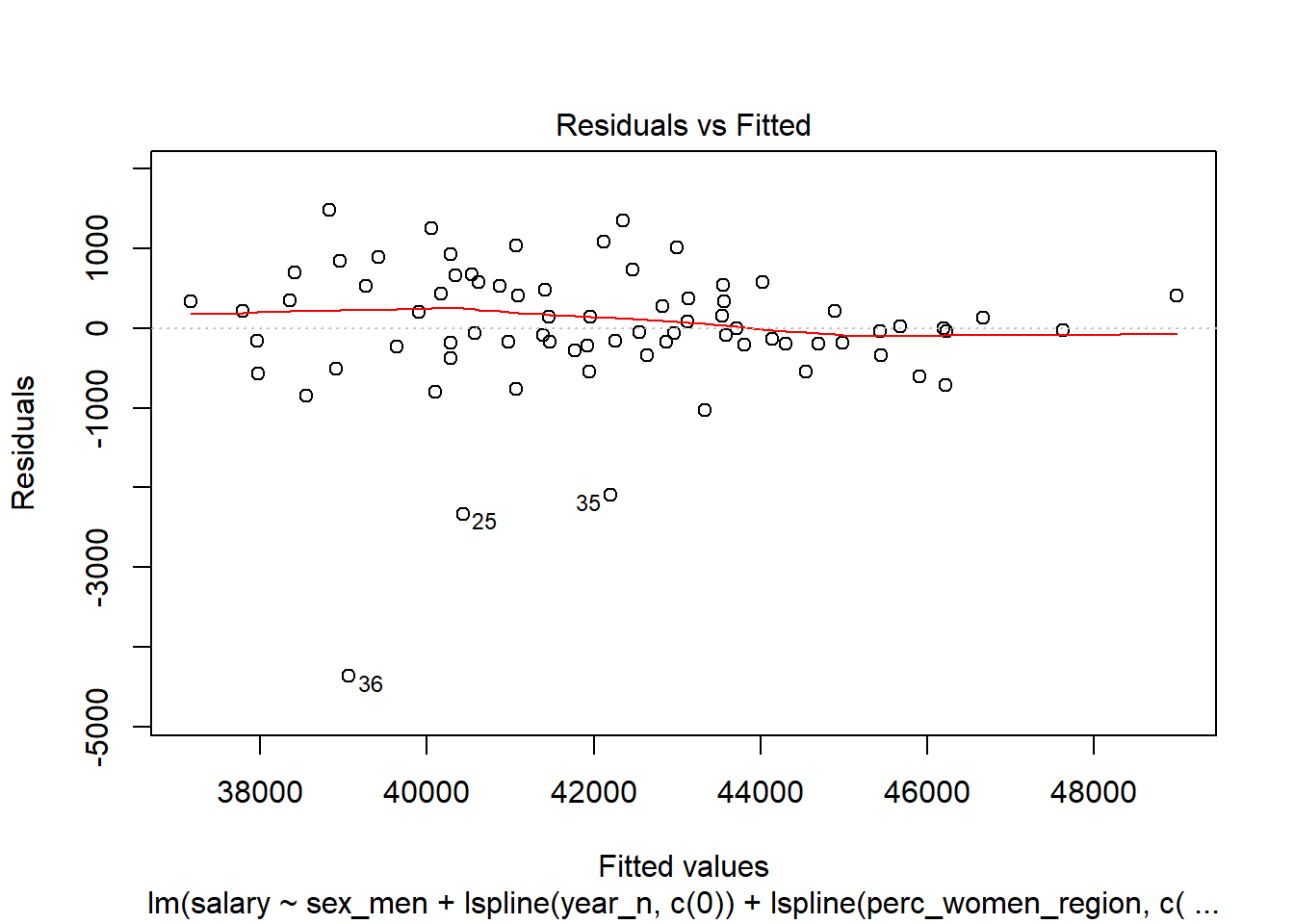
Figure 13: Diagnostics on the model, Year 2014 - 2018
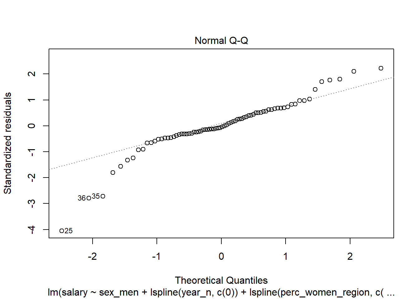
Figure 14: Diagnostics on the model, Year 2014 - 2018
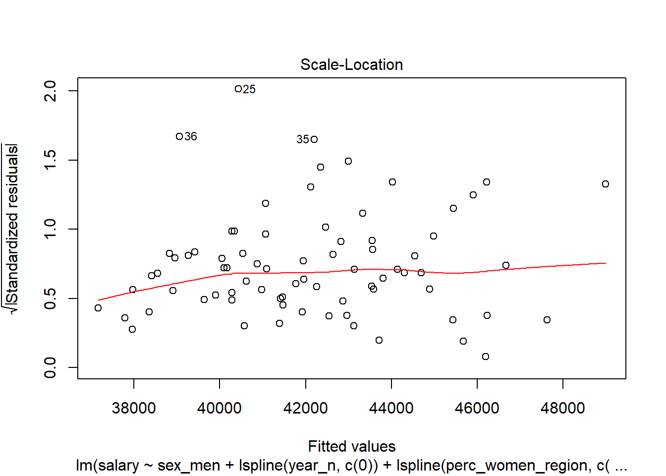
Figure 15: Diagnostics on the model, Year 2014 - 2018
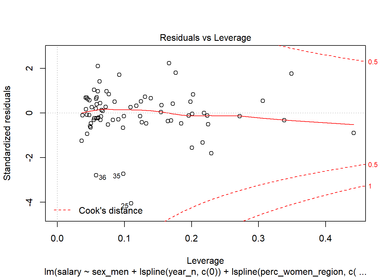
Figure 16: Diagnostics on the model, Year 2014 - 2018
binnedplot(predict(model), resid(model))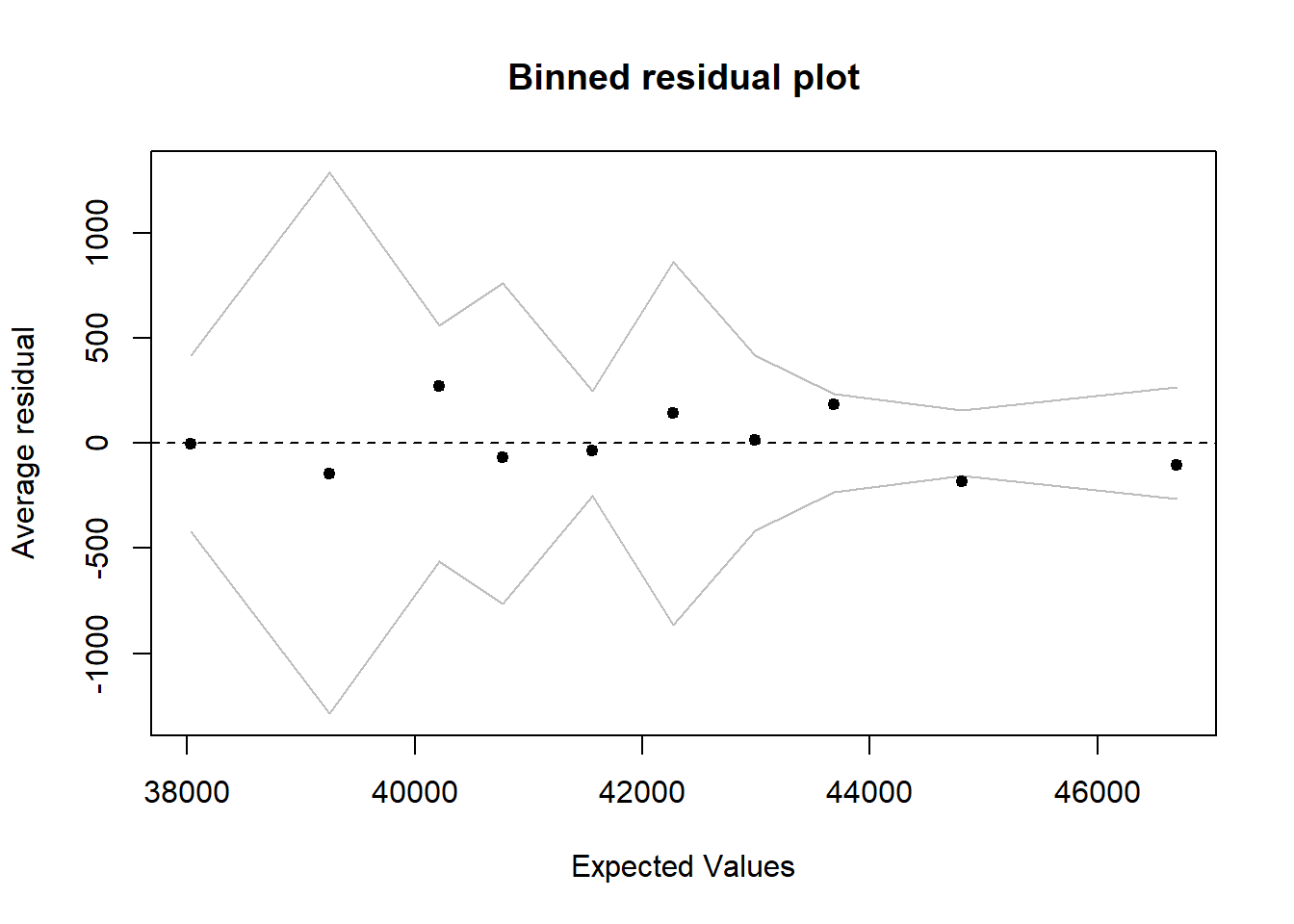
Figure 17: Diagnostics on the model, Year 2014 - 2018
halfnorm(rstudent(model))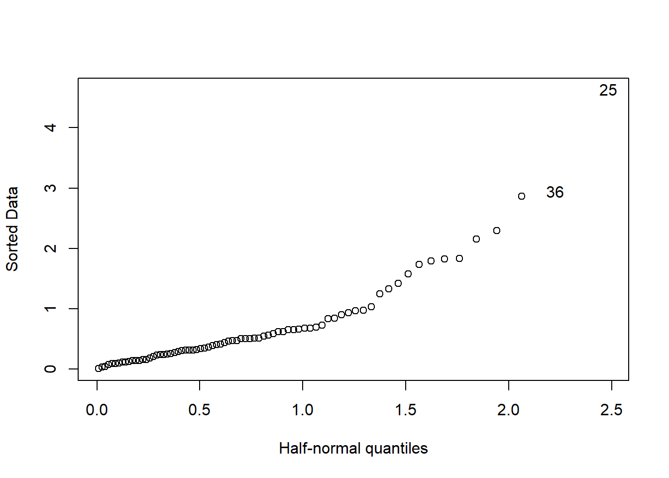
Figure 18: Diagnostics on the model, Year 2014 - 2018
tbnum %>% mutate(residuals = residuals(model)) %>%
  group_by(salary, perc_women_region, suming, year_n, sex_men) %>%
  summarise(residuals = mean(residuals), count = sum(suming)) %>%
    ggplot (aes(x = salary, y = residuals, size = sqrt(count), colour = perc_women_region)) +
    geom_point() + facet_grid(. ~ year_n)
## Warning in sqrt(count): NaNs produced
## Warning in sqrt(count): NaNs produced## Warning: Removed 49 rows containing missing values (geom_point).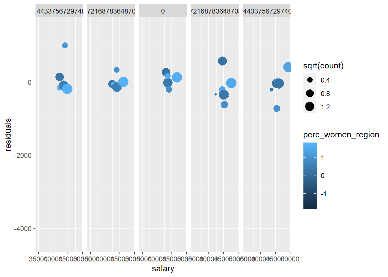
Figure 19: Diagnostics on the model, Year 2014 - 2018
set.seed(123)
results <- boot(data = tbnum, statistic = bs,
  R = 1000, formula = as.formula(model))

summary (model) %>% tidy() %>%
  mutate(bootest = tidy(results)$statistic,
  bootbias = tidy(results)$bias,
  booterr =  tidy(results)$std.error,
  conf = !((tidy(confint(results))$X2.5.. < 0) & (tidy(confint(results))$X97.5.. > 0)))
## Warning: 'tidy.matrix' is deprecated.
## See help("Deprecated")## Warning: 'tidy.matrix' is deprecated.
## See help("Deprecated")## # A tibble: 9 x 9
## term estimate std.error statistic p.value bootest bootbias booterr conf
## <chr> <dbl> <dbl> <dbl> <dbl> <dbl> <dbl> <dbl> <lgl>
## 1 (Interce~ 41613. 1045. 39.8 2.33e-48 41613. 50.1 1258. TRUE
## 2 sex_men 1806. 252. 7.15 8.00e-10 1806. -5.79 402. TRUE
## 3 lspline(~ 949. 136. 6.99 1.56e- 9 949. -99.1 358. TRUE
## 4 lspline(~ 1694. 131. 12.9 7.16e-20 1694. 26.7 329. TRUE
## 5 lspline(~ 1482. 238. 6.22 3.72e- 8 1482. 10.7 326. TRUE
## 6 lspline(~ 1532. 136. 11.2 4.88e-17 1532. -119. 241. TRUE
## 7 lspline(~ 1625. 1734. 0.937 3.52e- 1 1625. 118. 2169. FALSE
## 8 lspline(~ 409. 112. 3.65 5.20e- 4 409. 19.5 196. TRUE
## 9 sex_men:~ -516. 89.7 -5.75 2.44e- 7 -516. 12.3 246. TRUEplot(results, index = 1) # intercept 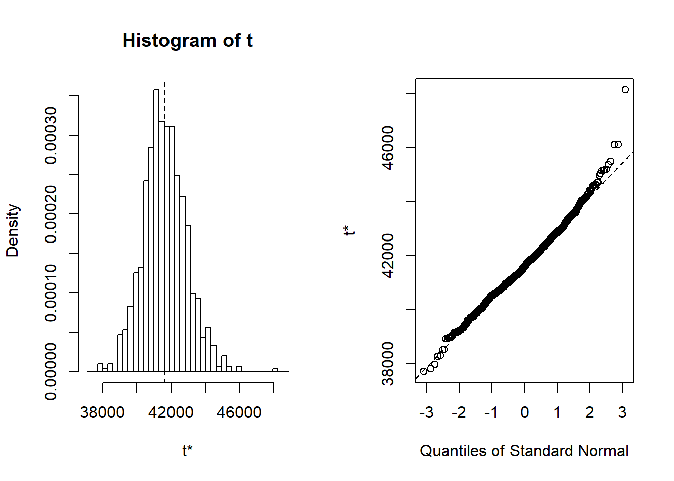
Figure 20: Diagnostics on the model, Year 2014 - 2018
Let’s have a look at the outliers.
tb_outliers_info[25,]## # A tibble: 1 x 11
## region salary year_n regiongroupsize sex regioneduyears suming
## <chr> <dbl> <dbl> <dbl> <chr> <dbl> <dbl>
## 1 SE31 ~ 38100 2015 304987 men 11.2 4600
## # ... with 4 more variables: perc_women_region <dbl>, salaryquotient <dbl>,
## # eduquotient <dbl>, perc_women_eng_region <dbl>tb_outliers_info[35,]## # A tibble: 1 x 11
## region salary year_n regiongroupsize sex regioneduyears suming
## <chr> <dbl> <dbl> <dbl> <chr> <dbl> <dbl>
## 1 SE21 ~ 40100 2016 304366 men 11.3 2600
## # ... with 4 more variables: perc_women_region <dbl>, salaryquotient <dbl>,
## # eduquotient <dbl>, perc_women_eng_region <dbl>tb_outliers_info[36,]## # A tibble: 1 x 11
## region salary year_n regiongroupsize sex regioneduyears suming
## <chr> <dbl> <dbl> <dbl> <chr> <dbl> <dbl>
## 1 SE21 ~ 34700 2016 290140 women 11.7 660
## # ... with 4 more variables: perc_women_region <dbl>, salaryquotient <dbl>,
## # eduquotient <dbl>, perc_women_eng_region <dbl>Now let’s see what we have found. I will plot both the regression and the decision trees models for comparison.
temp <- dplyr::select(tb_unique, c(salary, year_n, sex, perc_women_region, suming, salaryquotient, regioneduyears))

mmod <- earth(salary ~ ., weights = tbnum_weights, data = temp, nk = 11, degree = 2)

summary(mmod)
## Call: earth(formula=salary~., data=temp, weights=tbnum_weights, degree=2,
## nk=11)
##
## coefficients
## (Intercept) 43393.134
## sexwomen -1907.433
## h(2016-year_n) -704.320
## h(year_n-2016) 1184.617
## h(0.493906-perc_women_region) -250482.793
## h(perc_women_region-0.493906) 295538.165
## h(suming-2400) 0.067
## h(0.925101-salaryquotient) -31088.734
## h(salaryquotient-0.925101) -18920.288
##
## Selected 9 of 10 terms, and 5 of 6 predictors
## Termination condition: Reached nk 11
## Importance: year_n, suming, perc_women_region, sexwomen, salaryquotient, ...
## Weights: 21400, 6800, 11500, 3000, 2400, 500, 7000, 1900, 16000, 4100, 3...
## Number of terms at each degree of interaction: 1 8 (additive model)
## GCV 3188847459 RSS 126924520583 GRSq 0.9055366 RSq 0.9491997model <- lm (salary ~
sex +
lspline(year_n, c(2016)) +
lspline(perc_women_region, c(0.493906)) +
lspline(suming, c(2400)) +
sex:salaryquotient,
weights = tbnum_weights,
data = tb_unique)
set.seed(123) # for reproducibility
tbnum_bag <- train(
salary ~ .,
data = tb_unique,
method = "treebag",
weights = suming,
trControl = trainControl(method = "cv", number = 10),
nbagg = 200,
control = rpart.control(minsplit = 2, cp = 0)
)
p1 <- plot_model (model, type = "pred", terms = c("perc_women_region"))
p2 <- partial(tbnum_bag, pred.var = "perc_women_region") %>% autoplot()
gridExtra::grid.arrange(p1, p2, ncol = 2)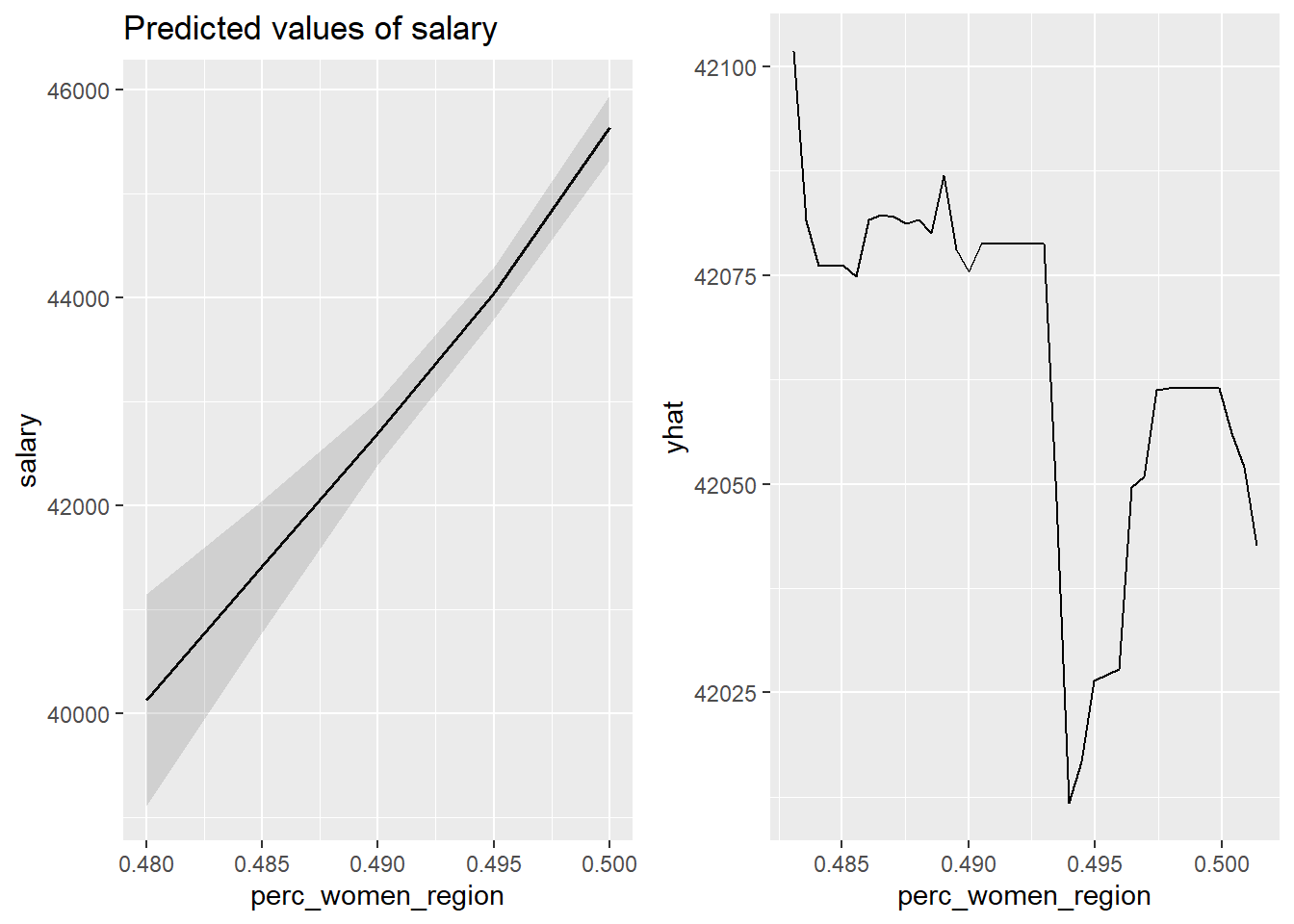
Figure 21: The significance of the per cent women in the region on the salary for engineers, Year 2014 - 2018
tb_unique %>%
  ggplot () +
    geom_jitter (mapping = aes(x = perc_women_region, y = salary)) +
  labs(
    x = "Percent women in region",
    y = "Salary"
  )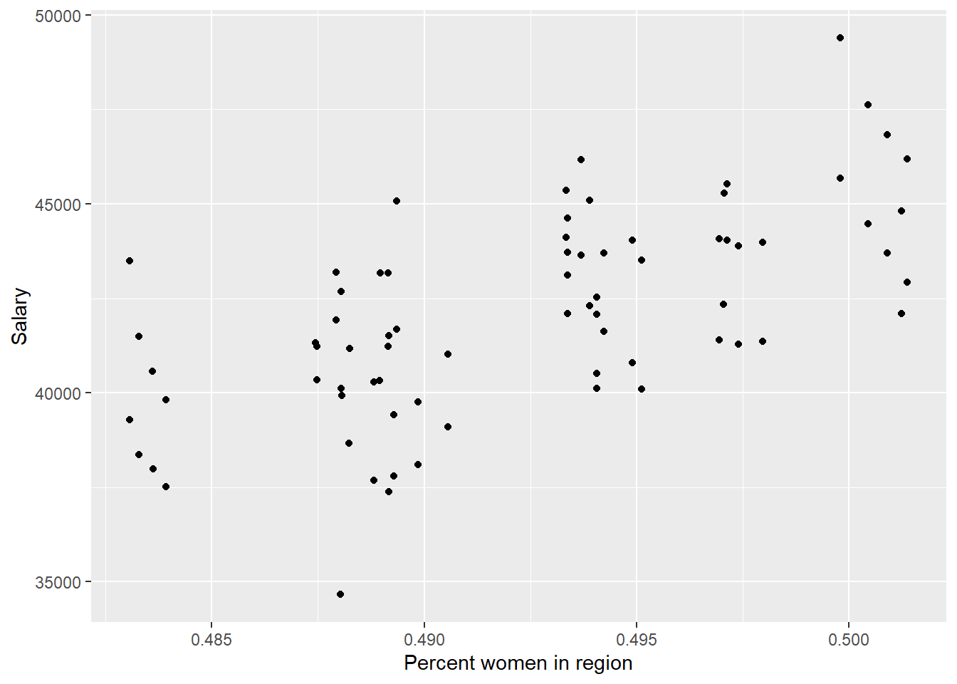
Figure 22: The significance of the per cent women in the region on the salary for engineers, Year 2014 - 2018
p1 <- plot_model (model, type = "pred", terms = c("year_n"))

p2 <- partial(tbnum_bag, pred.var = "year_n") %>% autoplot()

gridExtra::grid.arrange(p1, p2, ncol = 2)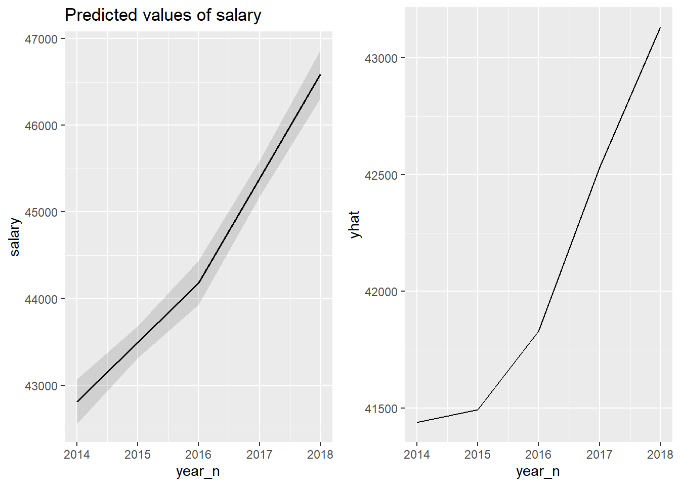
Figure 23: The significance of the year on the salary for engineers, Year 2014 - 2018
tb_unique %>%
  ggplot () +
    geom_jitter (mapping = aes(x = year_n, y = salary)) +
  labs(
    x = "Year",
    y = "Salary"
  )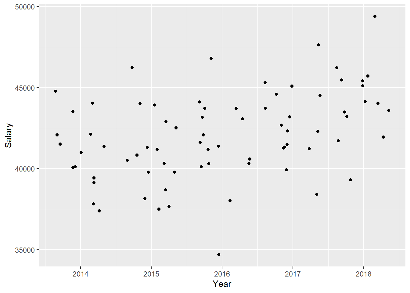
Figure 24: The significance of the year on the salary for engineers, Year 2014 - 2018
p1 <- plot_model (model, type = "pred", terms = c("sex"))

p2 <- tb_unique %>%
  ggplot () +
    geom_jitter (mapping = aes(x = sex, y = salary)) +
  labs(
    x = "Sex",
    y = "Salary"
  )

gridExtra::grid.arrange(p1, p2, ncol = 2)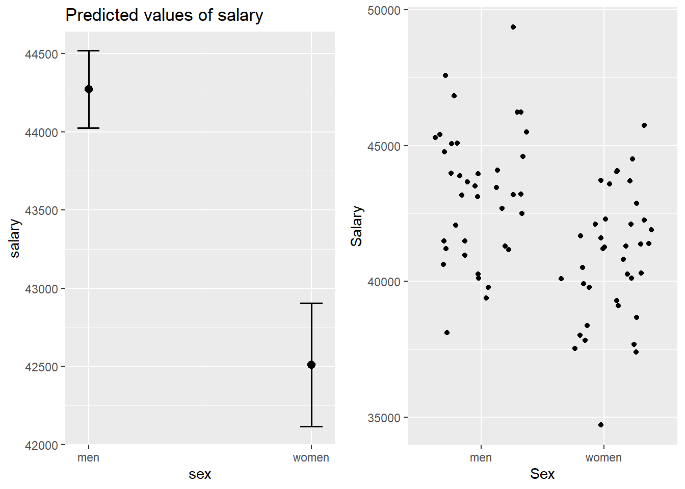
Figure 25: The significance of gender on the salary for engineers, Year 2014 - 2018
p1 <- plot_model (model, type = "pred", terms = c("suming"))

p2 <- partial(tbnum_bag, pred.var = "suming") %>% autoplot()

gridExtra::grid.arrange(p1, p2, ncol = 2)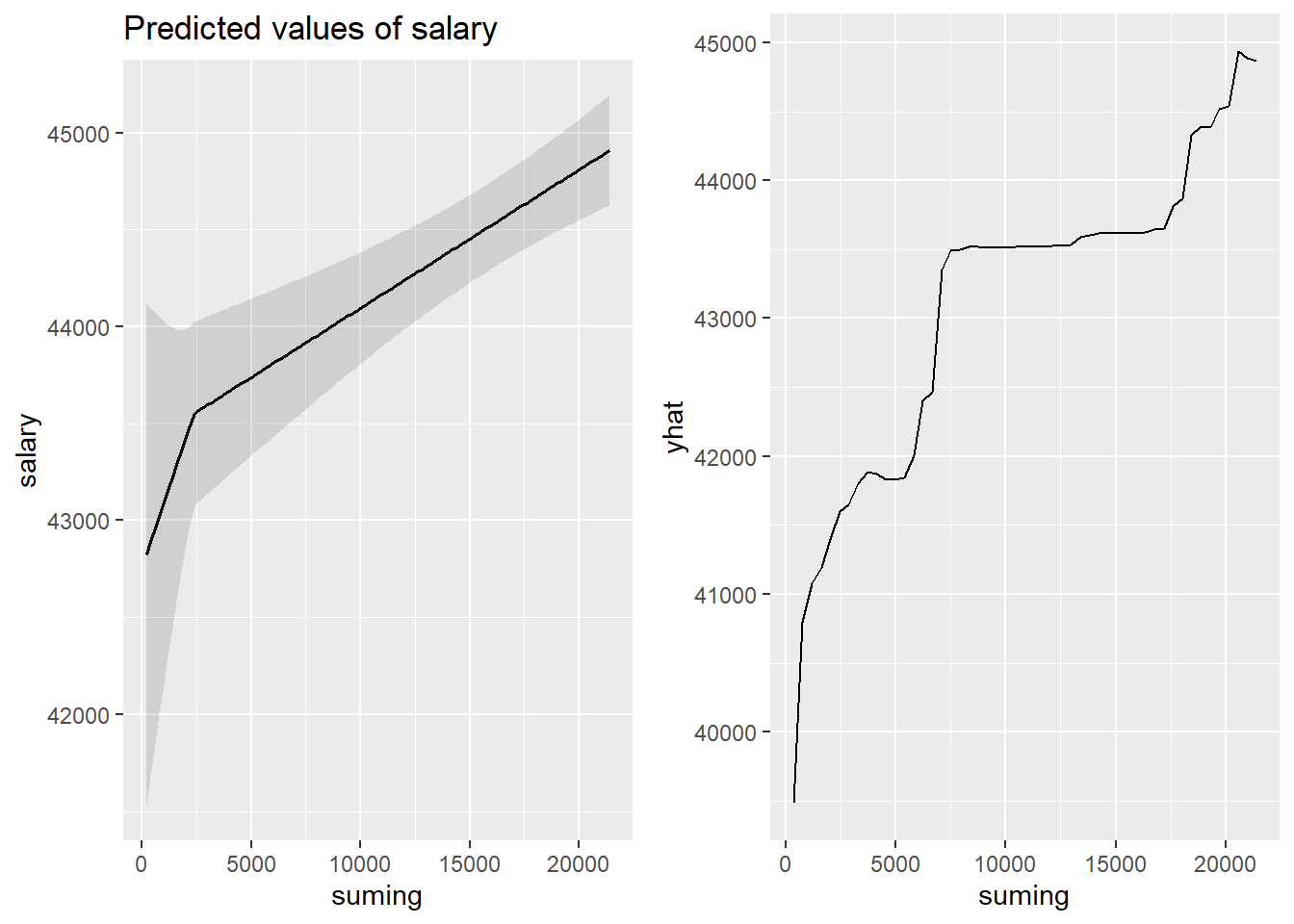
Figure 26: The significance of the number of engineers on the salary for engineers, Year 2014 - 2018
tb_unique %>%
  ggplot () +
    geom_jitter (mapping = aes(x = suming, y = salary)) +
  labs(
    x = "# engineers in the region",
    y = "Salary"
  )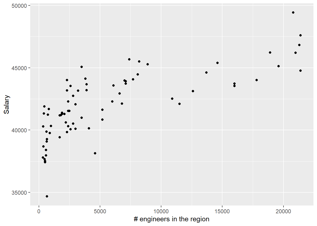
Figure 27: The significance of the number of engineers on the salary for engineers, Year 2014 - 2018
p1 <- plot_model (model, type = "pred", terms = c("salaryquotient", "sex"))

p2 <- tb_unique %>%
  ggplot () +
    geom_jitter (mapping = aes(x = salaryquotient, y = salary, colour = sex)) +
  labs(
    x = "Quotient between salary for men and women",
    y = "Salary"
  )

gridExtra::grid.arrange(p1, p2, ncol = 2)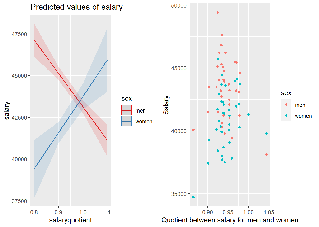
Figure 28: The significance of the interaction between sex and the quotient between salary for men and women within each group defined by year and region on the salary for engineers, Year 2014 - 2018
p1 <- plot_model (model, type = "pred", terms = c("year_n", "sex"))

p2 <- tb_unique %>%
  ggplot () +
    geom_jitter (mapping = aes(x = year_n, y = salary, colour = sex)) +
  labs(
    x = "Year",
    y = "Salary"
  )

gridExtra::grid.arrange(p1, p2, ncol = 2)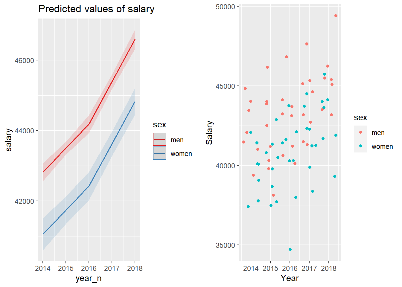
Figure 29: The combination of the year and sex on the salary for engineers, Year 2014 - 2018
p1 <- plot_model (model, type = "pred", terms = c("perc_women_region", "sex"))

p2 <- tb_unique %>%
  ggplot () +
    geom_jitter (mapping = aes(x = perc_women_region, y = salary, colour = sex)) +
  labs(
    x = "Percent women in region",
    y = "Salary"
  )

gridExtra::grid.arrange(p1, p2, ncol = 2)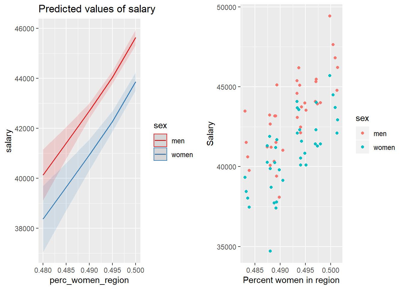
Figure 30: The combination of the per cent women in the region and sex on the salary for engineers, Year 2014 - 2018
p1 <- plot_model (model, type = "pred", terms = c("suming", "sex"))

p2 <- tb_unique %>%
  ggplot () +
    geom_jitter (mapping = aes(x = suming, y = salary, colour = sex)) +
  labs(
    x = "# engineers in the region",
    y = "Salary"
  )

gridExtra::grid.arrange(p1, p2, ncol = 2)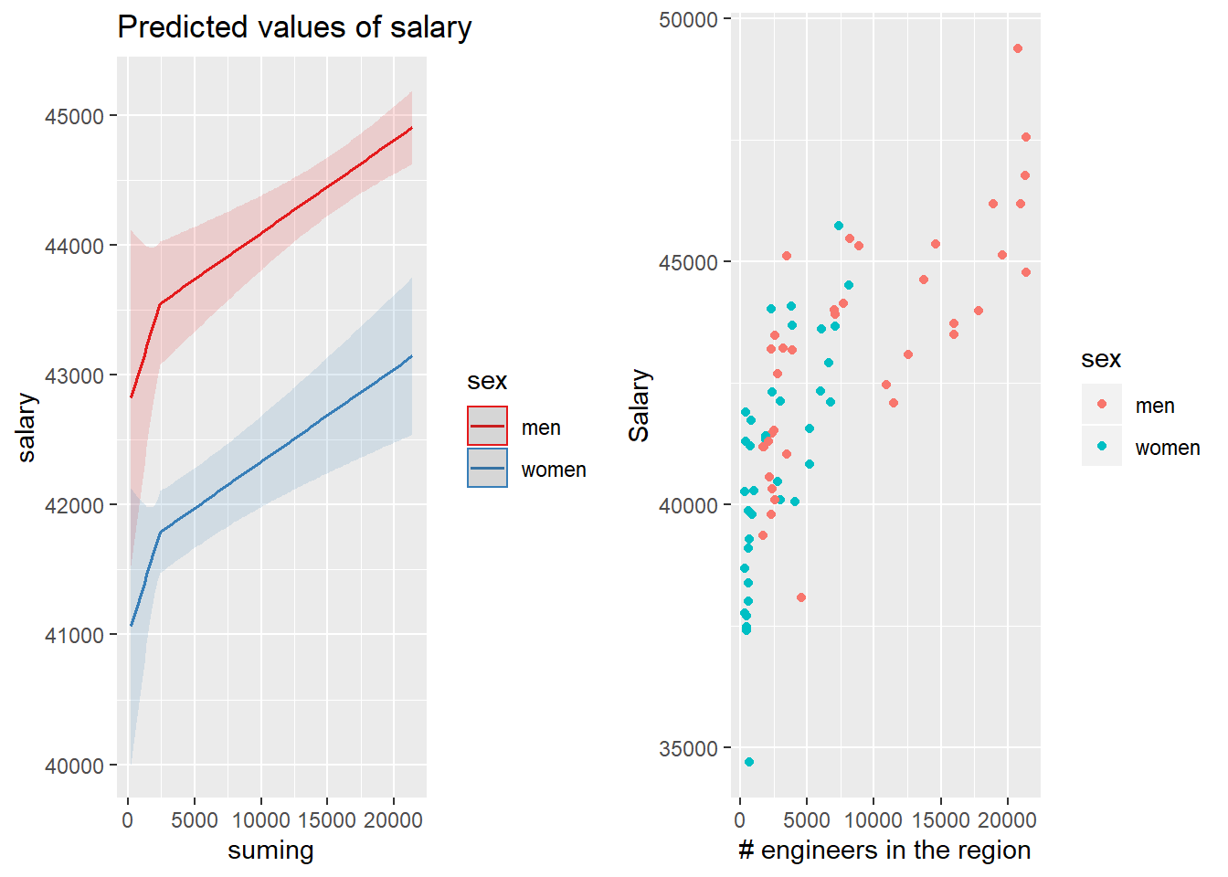
Figure 31: The combination of the number of engineers in the region and sex on the salary for engineers, Year 2014 - 2018
p1 <- plot_model (model, type = "pred", terms = c("year_n", "perc_women_region"))

p2 <- partial(tbnum_bag, pred.var = c("perc_women_region", "year_n")) %>%
  plotPartial(levelplot = FALSE, zlab = "yhat", drape = TRUE,
              colorkey = TRUE, screen = list(z = -20, x = -60))

gridExtra::grid.arrange(p1, p2, ncol = 2)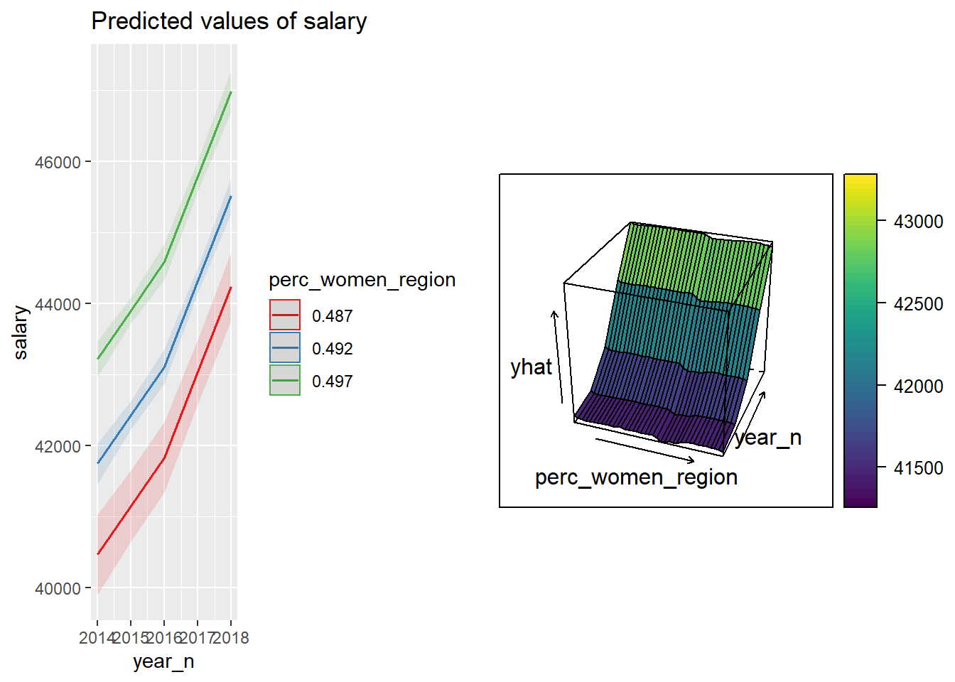
Figure 32: The combination of the year and per cent women in the region on the salary for engineers, Year 2014 - 2018
tb_unique %>%
  ggplot () +
    geom_jitter (mapping = aes(x = year_n, y = salary, colour = perc_women_region)) +
  labs(
    x = "Year",
    y = "Salary"
  )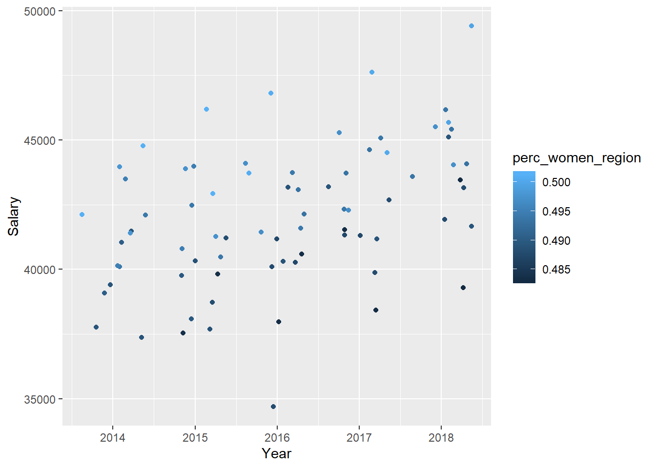
Figure 33: The combination of the year and per cent women in the region on the salary for engineers, Year 2014 - 2018
p1 <- plot_model (model, type = "pred", terms = c("year_n", "suming"))

p2 <- partial(tbnum_bag, pred.var = c("suming", "year_n")) %>%
  plotPartial(levelplot = FALSE, zlab = "yhat", drape = TRUE,
              colorkey = TRUE, screen = list(z = -20, x = -60))

gridExtra::grid.arrange(p1, p2, ncol = 2)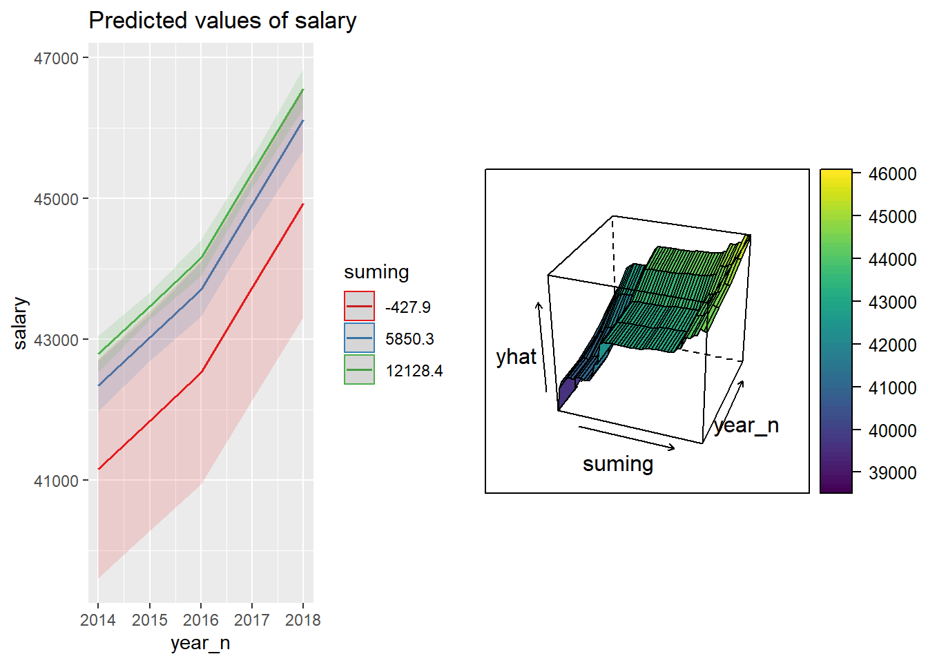
Figure 34: The combination of the year and number of engineers in the region on the salary for engineers, Year 2014 - 2018
tb_unique %>%
  ggplot () +
    geom_jitter (mapping = aes(x = year_n, y = salary, colour = suming)) +
  labs(
    x = "Year",
    y = "Salary"
  )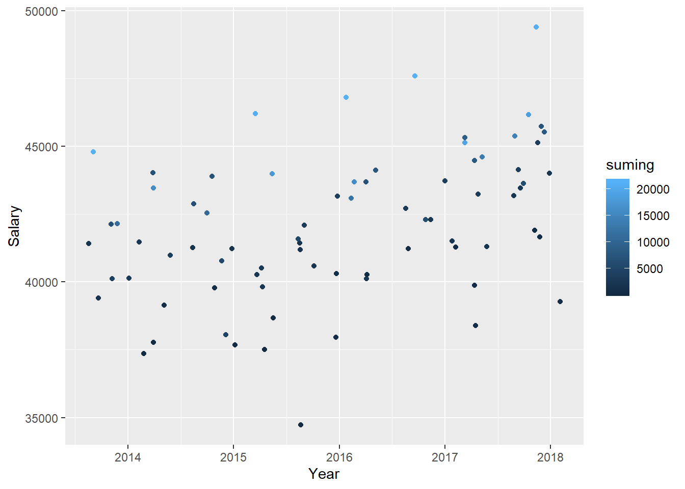
Figure 35: The combination of the year and number of engineers in the region on the salary for engineers, Year 2014 - 2018
p1 <- plot_model (model, type = "pred", terms = c("suming", "perc_women_region"))

p2 <- partial(tbnum_bag, pred.var = c("perc_women_region", "suming")) %>%
  plotPartial(levelplot = FALSE, zlab = "yhat", drape = TRUE,
              colorkey = TRUE, screen = list(z = -20, x = -60))

gridExtra::grid.arrange(p1, p2, ncol = 2)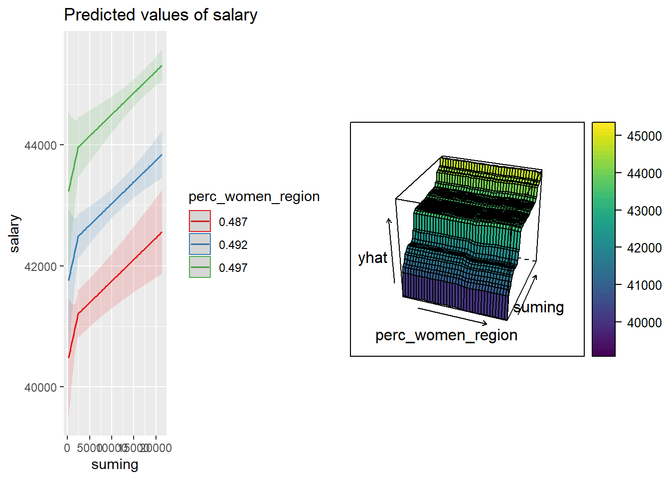
Figure 36: The combination of the number of engineers in the region and per cent women in the region on the salary for engineers, Year 2014 - 2018
tb_unique %>%
  ggplot () +
    geom_jitter (mapping = aes(x = suming, y = salary, colour = perc_women_region)) +
  labs(
    x = "# engineers in the region",
    y = "Salary"
  )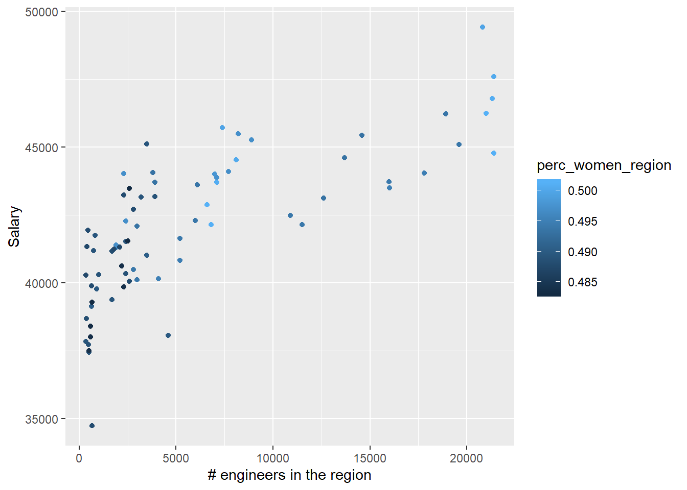
Figure 37: The combination of the number of engineers in the region and per cent women in the region on the salary for engineers, Year 2014 - 2018