In my last post, I found that the per cent women in the region had a significant impact on the salaries of Engineers. In this post, I will analyse what predictors are best to forecast the percentage of women who are Engineers in the region. I will begin in much the same way as when I looked at salaries. However, there are limitations to linear models. In the second half of this post, I compare my finding to other machine learning algorithms.
Statistics Sweden use NUTS (Nomenclature des Unités Territoriales Statistiques), which is the EU’s hierarchical regional division, to specify the regions.
Please send suggestions for improvement of the analysis to ranalystatisticssweden@gmail.com.
First, define libraries and functions.
library (tidyverse)## -- Attaching packages -------------------------------------------------- tidyverse 1.3.0 --## v ggplot2 3.3.0 v purrr 0.3.4
## v tibble 3.0.0 v dplyr 0.8.5
## v tidyr 1.0.2 v stringr 1.4.0
## v readr 1.3.1 v forcats 0.5.0## -- Conflicts ----------------------------------------------------- tidyverse_conflicts() --
## x dplyr::filter() masks stats::filter()
## x dplyr::lag() masks stats::lag()library (broom)
library (car)## Loading required package: carData##
## Attaching package: 'car'## The following object is masked from 'package:dplyr':
##
## recode## The following object is masked from 'package:purrr':
##
## somelibrary (leaps)
library (MASS)##
## Attaching package: 'MASS'## The following object is masked from 'package:dplyr':
##
## selectlibrary (earth)## Loading required package: Formula## Loading required package: plotmo## Loading required package: plotrix## Loading required package: TeachingDemoslibrary (lspline)
library (boot)##
## Attaching package: 'boot'## The following object is masked from 'package:car':
##
## logitlibrary (arm)## Loading required package: Matrix##
## Attaching package: 'Matrix'## The following objects are masked from 'package:tidyr':
##
## expand, pack, unpack## Loading required package: lme4## Registered S3 methods overwritten by 'lme4':
## method from
## cooks.distance.influence.merMod car
## influence.merMod car
## dfbeta.influence.merMod car
## dfbetas.influence.merMod car##
## arm (Version 1.10-1, built: 2018-4-12)## Working directory is C:/R/rblog/content/post##
## Attaching package: 'arm'## The following object is masked from 'package:boot':
##
## logit## The following object is masked from 'package:plotrix':
##
## rescale## The following object is masked from 'package:car':
##
## logitlibrary (caret) ## Loading required package: lattice##
## Attaching package: 'lattice'## The following object is masked from 'package:boot':
##
## melanoma##
## Attaching package: 'caret'## The following object is masked from 'package:purrr':
##
## liftlibrary (recipes) ##
## Attaching package: 'recipes'## The following object is masked from 'package:stringr':
##
## fixed## The following object is masked from 'package:stats':
##
## steplibrary (vip) ##
## Attaching package: 'vip'## The following object is masked from 'package:utils':
##
## vilibrary (ggpubr)## Loading required package: magrittr##
## Attaching package: 'magrittr'## The following object is masked from 'package:purrr':
##
## set_names## The following object is masked from 'package:tidyr':
##
## extractlibrary (glmnet)## Loaded glmnet 3.0-2library (rpart)
library (ipred)
library (iml)
library (neuralnet)##
## Attaching package: 'neuralnet'## The following object is masked from 'package:dplyr':
##
## computelibrary (DALEX)## Welcome to DALEX (version: 1.2.1).
## Find examples and detailed introduction at: https://pbiecek.github.io/ema/##
## Attaching package: 'DALEX'## The following object is masked from 'package:dplyr':
##
## explainlibrary (Metrics)##
## Attaching package: 'Metrics'## The following objects are masked from 'package:caret':
##
## precision, recalllibrary (auditor)##
## Attaching package: 'auditor'## The following object is masked from 'package:DALEX':
##
## model_performancereadfile <- function (file1){read_csv (file1, col_types = cols(), locale = readr::locale (encoding = "latin1"), na = c("..", "NA")) %>%
gather (starts_with("19"), starts_with("20"), key = "year", value = groupsize) %>%
drop_na() %>%
mutate (year_n = parse_number (year))
}
perc_women <- function(x){
ifelse (length(x) == 2, x[2] / (x[1] + x[2]), NA)
}
nuts <- read.csv("nuts.csv") %>%
mutate(NUTS2_sh = substr(NUTS2, 3, 4))
nuts %>%
distinct (NUTS2_en) %>%
knitr::kable(
booktabs = TRUE,
caption = 'Nomenclature des Unités Territoriales Statistiques (NUTS)')| NUTS2_en |
|---|
| SE11 Stockholm |
| SE12 East-Central Sweden |
| SE21 Småland and islands |
| SE22 South Sweden |
| SE23 West Sweden |
| SE31 North-Central Sweden |
| SE32 Central Norrland |
| SE33 Upper Norrland |
bs <- function(formula, data, indices) {
  d <- data[indices,] # allows boot to select sample
  fit <- lm(formula, weights = tbnum_weights, data=d)
  return(coef(fit))
}
The data tables are downloaded from Statistics Sweden. They are saved as a comma-delimited file without heading, UF0506A1.csv, http://www.statistikdatabasen.scb.se/pxweb/en/ssd/.
The tables:
UF0506A1_1.csv: Population 16-74 years of age by region, highest level of education, age and sex. Year 1985 - 2018 NUTS 2 level 2008- Age, total, all reported ages
000000CG_1: Average basic salary, monthly salary and women´s salary as a percentage of men´s salary by region, sector, occupational group (SSYK 2012) and sex. Year 2014 - 2018 Monthly salary All sectors.
000000CD_1.csv: Average basic salary, monthly salary and women´s salary as a percentage of men´s salary by region, sector, occupational group (SSYK 2012) and sex. Year 2014 - 2018 Number of employees All sectors-
The data is aggregated, the size of each group is in the column groupsize.
I have also included some calculated predictors from the original data.
perc_women: The percentage of women within each group defined by edulevel, region and year
perc_women_region: The percentage of women within each group defined by year and region
regioneduyears: The average number of education years per capita within each group defined by sex, year and region
eduquotient: The quotient between regioneduyears for men and women
salaryquotient: The quotient between salary for men and women within each group defined by year and region
perc_women_eng_region: The percentage of women who are engineers within each group defined by year and region
numedulevel <- read.csv("edulevel_1.csv")

numedulevel[, 2] <- data.frame(c(8, 9, 10, 12, 13, 15, 22, NA))

tb <- readfile("000000CG_1.csv")
tb <- readfile("000000CD_1.csv") %>%
  left_join(tb, by = c("region", "year", "sex", "sector","occuptional  (SSYK 2012)")) %>%
  filter(`occuptional  (SSYK 2012)` == "214 Engineering professionals")

tb <- readfile("UF0506A1_1.csv") %>%
  right_join(tb, by = c("region", "year", "sex")) %>%
  right_join(numedulevel, by = c("level of education" = "level.of.education")) %>%
  filter(!is.na(eduyears)) %>%
  mutate(edulevel = `level of education`) %>%
  group_by(edulevel, region, year, sex) %>%
  mutate(groupsize_all_ages = sum(groupsize)) %>%
  group_by(edulevel, region, year) %>%
  mutate (perc_women = perc_women (groupsize_all_ages[1:2])) %>%
  group_by (sex, year, region) %>%
  mutate(regioneduyears = sum(groupsize * eduyears) / sum(groupsize)) %>%
  mutate(regiongroupsize = sum(groupsize)) %>%
  mutate(suming = groupsize.x) %>%
  group_by(region, year) %>%
  mutate (sum_pop = sum(groupsize)) %>%
  mutate (perc_women_region = perc_women (regiongroupsize[1:2])) %>%
  mutate (eduquotient = regioneduyears[2] / regioneduyears[1]) %>%
  mutate (salary = groupsize.y) %>%
  mutate (salaryquotient = salary[2] / salary[1]) %>%
  mutate (perc_women_eng_region = perc_women(suming[1:2])) %>%
  left_join(nuts %>% distinct (NUTS2_en, NUTS2_sh), by = c("region" = "NUTS2_en")) %>%
  drop_na()

summary(tb)
## region age level of education sex
## Length:532 Length:532 Length:532 Length:532
## Class :character Class :character Class :character Class :character
## Mode :character Mode :character Mode :character Mode :character
##
##
##
## year groupsize year_n sector
## Length:532 Min. : 405 Min. :2014 Length:532
## Class :character 1st Qu.: 20996 1st Qu.:2015 Class :character
## Mode :character Median : 43656 Median :2016 Mode :character
## Mean : 64760 Mean :2016
## 3rd Qu.:102394 3rd Qu.:2017
## Max. :271889 Max. :2018
## occuptional (SSYK 2012) groupsize.x year_n.x groupsize.y
## Length:532 Min. : 340 Min. :2014 Min. :34700
## Class :character 1st Qu.: 1700 1st Qu.:2015 1st Qu.:40300
## Mode :character Median : 3000 Median :2016 Median :42000
## Mean : 5850 Mean :2016 Mean :42078
## 3rd Qu.: 7475 3rd Qu.:2017 3rd Qu.:43925
## Max. :21400 Max. :2018 Max. :49400
## year_n.y eduyears edulevel groupsize_all_ages
## Min. :2014 Min. : 8.00 Length:532 Min. : 405
## 1st Qu.:2015 1st Qu.: 9.00 Class :character 1st Qu.: 20996
## Median :2016 Median :12.00 Mode :character Median : 43656
## Mean :2016 Mean :12.71 Mean : 64760
## 3rd Qu.:2017 3rd Qu.:15.00 3rd Qu.:102394
## Max. :2018 Max. :22.00 Max. :271889
## perc_women regioneduyears regiongroupsize suming
## Min. :0.3575 Min. :11.18 Min. :128262 Min. : 340
## 1st Qu.:0.4338 1st Qu.:11.61 1st Qu.:288058 1st Qu.: 1700
## Median :0.4631 Median :11.74 Median :514608 Median : 3000
## Mean :0.4771 Mean :11.79 Mean :453318 Mean : 5850
## 3rd Qu.:0.5132 3rd Qu.:12.04 3rd Qu.:691870 3rd Qu.: 7475
## Max. :0.6423 Max. :12.55 Max. :827940 Max. :21400
## sum_pop perc_women_region eduquotient salary
## Min. : 262870 Min. :0.4831 Min. :1.019 Min. :34700
## 1st Qu.: 587142 1st Qu.:0.4882 1st Qu.:1.029 1st Qu.:40300
## Median :1029820 Median :0.4934 Median :1.034 Median :42000
## Mean : 906635 Mean :0.4923 Mean :1.034 Mean :42078
## 3rd Qu.:1395157 3rd Qu.:0.4970 3rd Qu.:1.041 3rd Qu.:43925
## Max. :1655215 Max. :0.5014 Max. :1.047 Max. :49400
## salaryquotient perc_women_eng_region NUTS2_sh
## Min. :0.8653 Min. :0.1566 Length:532
## 1st Qu.:0.9329 1st Qu.:0.1787 Class :character
## Median :0.9395 Median :0.2042 Mode :character
## Mean :0.9447 Mean :0.2039
## 3rd Qu.:0.9537 3rd Qu.:0.2216
## Max. :1.0446 Max. :0.2746Prepare the data using Tidyverse recipes package, i.e. centre, scale and make sure all predictors are numerical.
tbtemp <- ungroup(tb) %>% dplyr::select(region, salary, year_n, regiongroupsize, sex, regioneduyears, suming, perc_women_region, salaryquotient, eduquotient, perc_women_eng_region)

tb_outliers_info <- unique(tbtemp)

tb_unique <- unique(dplyr::select(tbtemp, -region))

tbnum_weights <- tb_unique$suming

blueprint <- recipe(perc_women_eng_region ~ ., data = tb_unique) %>%
  step_nzv(all_nominal()) %>%
  step_integer(matches("Qual|Cond|QC|Qu")) %>%
  step_center(all_numeric(), -all_outcomes()) %>%
  step_scale(all_numeric(), -all_outcomes()) %>%
  step_dummy(all_nominal(), -all_outcomes(), one_hot = TRUE)

prepare <- prep(blueprint, training = tb_unique)

tbnum <- bake(prepare, new_data = tb_unique)
The dataset only contains 76 rows. This together with multicollinearity limits the number of predictors to include in the regression. I would like to choose the predictors that best contains most information from the dataset with respect to the response.
I will use an elastic net to find the variable that contains the best signals for later use in the analysis. First I will search for the explanatory variables that best predict the response using no interactions. I will use 10-fold cross-validation with an elastic net. Elastic nets are linear and do not take into account the shape of the relations between the predictors. Alpha = 1 indicates a lasso regression.
X <- model.matrix(perc_women_eng_region ~ ., tbnum)[, -1]

Y <- tbnum$perc_women_eng_region

set.seed(123)  # for reproducibility
tbnum_glmnet <- caret::train(
    x = X,
    y = Y,
    weights = tbnum_weights,
    method = "glmnet",
    preProc = c("zv", "center", "scale"),
    trControl = trainControl(method = "cv", number = 10),
    tuneLength = 20
)
## Warning in nominalTrainWorkflow(x = x, y = y, wts = weights, info = trainInfo, :
## There were missing values in resampled performance measures.vip(tbnum_glmnet, num_features = 20, geom = "point")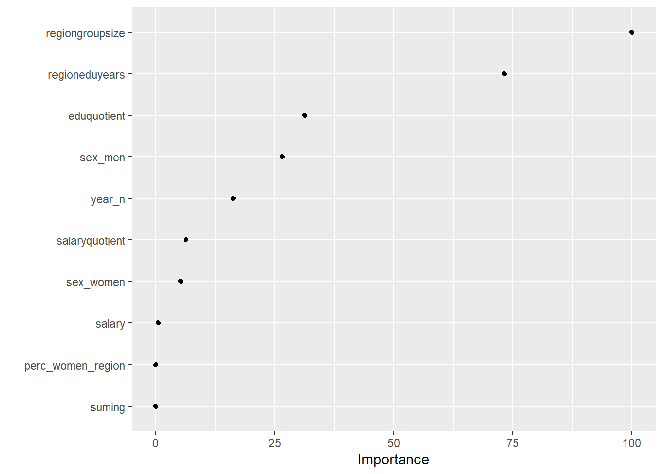
Figure 1: Elastic net search on the data using no interactions, Year 2014 - 2018
tbnum_glmnet$bestTune## alpha lambda
## 349 0.9052632 0.0002658605elastic_min <- glmnet(
x = X,
y = Y,
alpha = .1
)
plot(elastic_min, xvar = "lambda", main = "Elastic net penalty\n\n")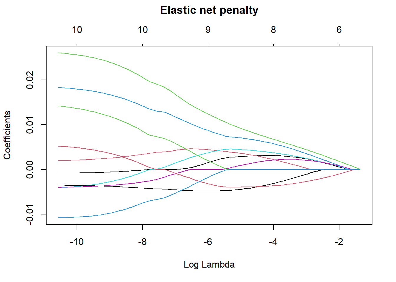
Figure 2: Elastic net search on the data using no interactions, Year 2014 - 2018
I use MARS to fit the best signals using from the elastic net using no interactions. Four predictors minimise the AIC while still ensuring that the coefficients are valid, testing them with bootstrap.
temp <- dplyr::select(tbnum, c(perc_women_eng_region, regiongroupsize, regioneduyears, eduquotient, sex_men))

mmod_scaled <- earth(perc_women_eng_region ~ ., weights = tbnum_weights, data = temp, nk = 9, degree = 1)

summary (mmod_scaled)
## Call: earth(formula=perc_women_eng_region~., data=temp, weights=tbnum_weights,
## degree=1, nk=9)
##
## coefficients
## (Intercept) 0.188579073
## sex_men 0.020170708
## h(0.651904-regiongroupsize) -0.017635288
## h(regiongroupsize-0.651904) 0.032588077
## h(-0.259811-regioneduyears) -0.021971561
## h(regioneduyears- -0.259811) 0.021625566
## h(-1.22297-eduquotient) -0.049922858
## h(eduquotient- -1.22297) 0.009477773
##
## Selected 8 of 8 terms, and 4 of 4 predictors
## Termination condition: Reached nk 9
## Importance: regiongroupsize, regioneduyears, eduquotient, sex_men
## Weights: 21400, 6800, 11500, 3000, 2400, 500, 7000, 1900, 16000, 4100, 3...
## Number of terms at each degree of interaction: 1 7 (additive model)
## GCV 0.8258677 RSS 40.43492 GRSq 0.8250241 RSq 0.8842515plot (mmod_scaled)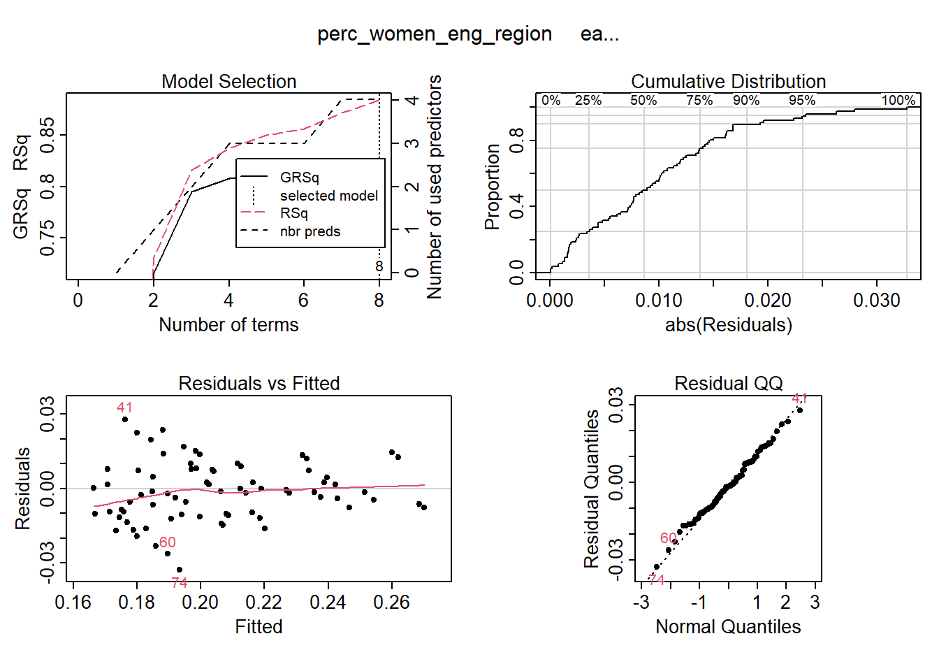
Figure 3: Hockey-stick functions fit with MARS for the predictors using no interactions, Year 2014 - 2018
plotmo (mmod_scaled)## plotmo grid: regiongroupsize regioneduyears eduquotient sex_men
## 0.2593006 -0.1394781 0 0.5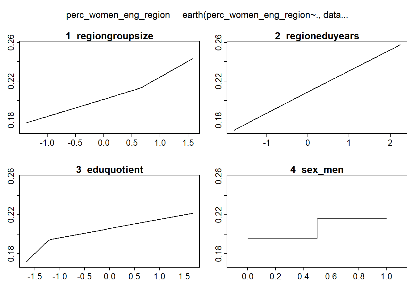
Figure 4: Hockey-stick functions fit with MARS for the predictors using no interactions, Year 2014 - 2018
model_mmod_scale <- lm (perc_women_eng_region ~
  sex_men +
  lspline(regiongroupsize, c(0.651904)) +
  lspline(regioneduyears, c(-0.259811)) +
  lspline(eduquotient, c(-1.22297)),
  weights = tbnum_weights,
  data = tbnum)

model_mmod_scale <- lm (perc_women_eng_region ~ .,
  weights = tbnum_weights,
  data = tbnum)

b <- regsubsets(perc_women_eng_region ~ sex_men + lspline(regiongroupsize, c(0.651904)) + lspline(regioneduyears, c(-0.259811)) + lspline(eduquotient, c(-1.22297)), data = tbnum, weights = tbnum_weights, nvmax = 12)

rs <- summary(b)
AIC <- 50 * log (rs$rss / 50) + (2:8) * 2
which.min (AIC)
## [1] 7names (rs$which[7,])[rs$which[7,]]## [1] "(Intercept)"
## [2] "sex_men"
## [3] "lspline(regiongroupsize, c(0.651904))1"
## [4] "lspline(regiongroupsize, c(0.651904))2"
## [5] "lspline(regioneduyears, c(-0.259811))1"
## [6] "lspline(regioneduyears, c(-0.259811))2"
## [7] "lspline(eduquotient, c(-1.22297))1"
## [8] "lspline(eduquotient, c(-1.22297))2"model_mmod_scale <- lm (perc_women_eng_region ~
sex_men +
lspline(regiongroupsize, c(0.651904)) +
lspline(regioneduyears, c(-0.259811)) +
lspline(eduquotient, c(-1.22297)),
weights = tbnum_weights,
data = tbnum)
summary (model_mmod_scale)$adj.r.squared## [1] 0.8723362AIC(model_mmod_scale)## [1] -426.1528set.seed(123)
results <- boot(data = tbnum, statistic = bs,
R = 1000, formula = as.formula(model_mmod_scale))
#conf = coefficient not passing through zero
summary (model_mmod_scale) %>% tidy() %>%
mutate(bootest = tidy(results)$statistic,
bootbias = tidy(results)$bias,
booterr = tidy(results)$std.error,
conf = !((tidy(confint(results))$X2.5.. < 0) & (tidy(confint(results))$X97.5.. > 0)))## Warning in norm.inter(t, adj.alpha): extreme order statistics used as endpoints## Warning: 'tidy.matrix' is deprecated.
## See help("Deprecated")## Warning in norm.inter(t, adj.alpha): extreme order statistics used as endpoints## Warning: 'tidy.matrix' is deprecated.
## See help("Deprecated")## # A tibble: 8 x 9
## term estimate std.error statistic p.value bootest bootbias booterr conf
## <chr> <dbl> <dbl> <dbl> <dbl> <dbl> <dbl> <dbl> <lgl>
## 1 (Interce~ 0.244 0.0177 13.8 2.05e-21 0.244 4.73e-3 0.0376 TRUE
## 2 sex_men 0.0202 0.00509 3.96 1.82e- 4 0.0202 2.44e-3 0.00694 TRUE
## 3 lspline(~ 0.0176 0.00437 4.03 1.42e- 4 0.0176 9.52e-4 0.00560 TRUE
## 4 lspline(~ 0.0326 0.00828 3.94 1.97e- 4 0.0326 -2.36e-3 0.0135 TRUE
## 5 lspline(~ 0.0220 0.00466 4.72 1.23e- 5 0.0220 -3.76e-3 0.00672 TRUE
## 6 lspline(~ 0.0216 0.00490 4.41 3.78e- 5 0.0216 4.59e-4 0.00672 TRUE
## 7 lspline(~ 0.0499 0.0133 3.76 3.56e- 4 0.0499 3.70e-3 0.0293 TRUE
## 8 lspline(~ 0.00948 0.00357 2.66 9.85e- 3 0.00948 -3.47e-3 0.00491 TRUEplot(results, index=1) # intercept 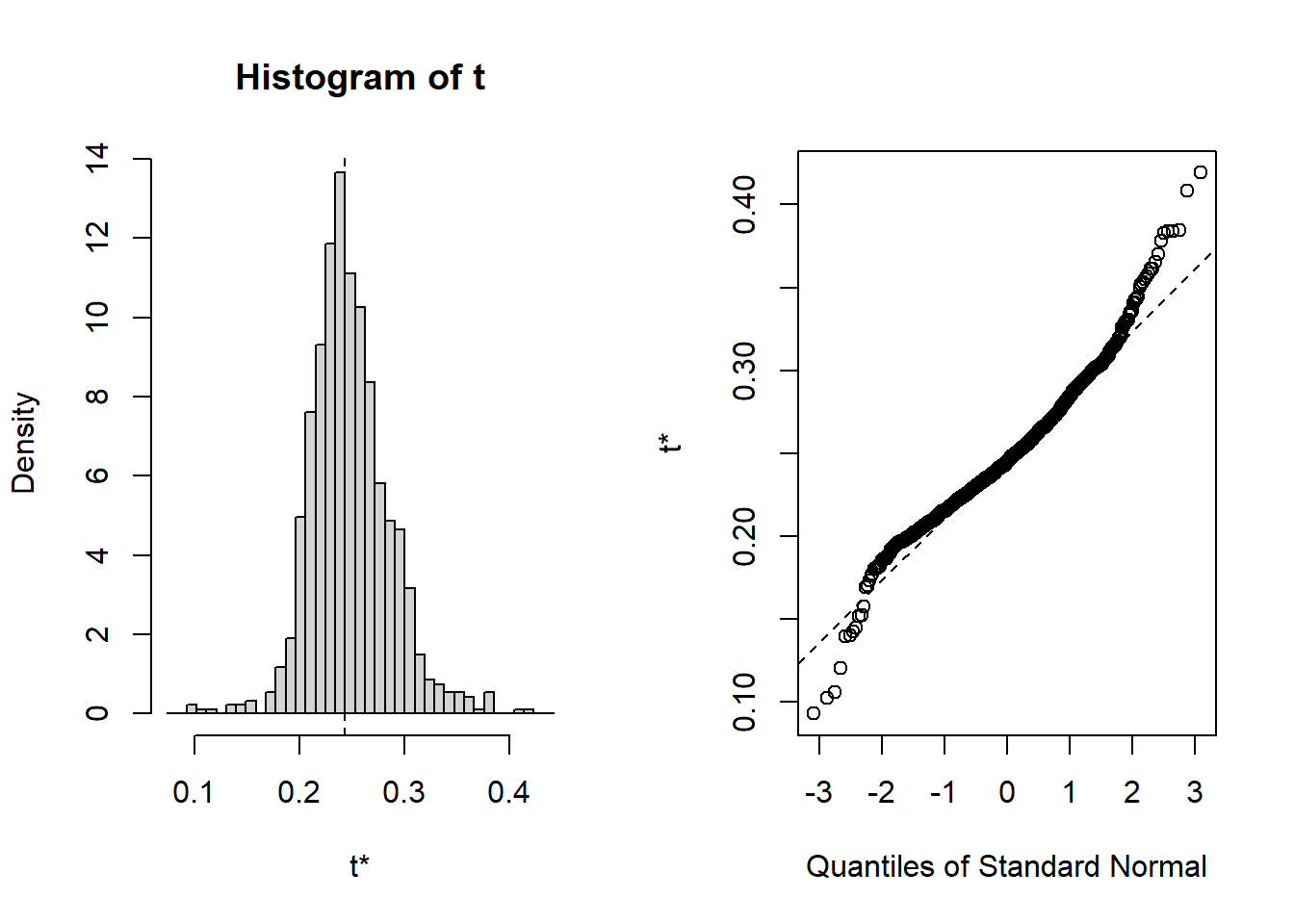
Figure 5: Hockey-stick functions fit with MARS for the predictors using no interactions, Year 2014 - 2018
plot_model will show diagnostics for the model, a residual plot, scale location plot, residual density and the regression error characteristic curve. It will also show the residuals versus the actual response to help find outliers. It will plot the feature importance and feature effects. In addition, it will plot how strongly features interact with each other and the 2-way interactions with regiongroupsize and all other features. The interaction measure regards how much of the variance of f(x) is explained by the interaction. The measure is between 0 (no interaction) and 1 (= 100% of variance of f(x) due to interactions). Regiongroupsize is of special interest since it is the feature with the strongest importance to the per cent of engineers who are women in the region.
plot_model <- function(model){
   invisible(capture.output(exp_model <- DALEX::explain(model, data = tbnum, y = tbnum$perc_women_eng_region))) # Knit and DALEX::explain generates invalid rss feed

   lm_mr <- model_residual(exp_model)

   predictor <- Predictor$new(model,
      data = dplyr::select(tbnum, -perc_women_eng_region),
      y = tbnum$perc_women_eng_region)

   writeLines("")

   print(paste ("Model RMSE: ", rmse(predict(model), tbnum$perc_women_eng_region)))

   p1 <- plot(lm_mr, type = "residual")

   p2 <- plot(lm_mr, type = "scalelocation")

   p3 <- plot(lm_mr, type = "residual_density")

   p4 <- plot(lm_mr, type = "rec")

   print(gridExtra::grid.arrange(p1, p2, p3, p4, ncol = 2))

   print(plot_residual(lm_mr, variable = "_y_hat_", nlabel = 10))

   print(plot (FeatureImp$new(predictor, loss = "mae")))

   print(plot (FeatureEffects$new(predictor)))

   p1 <- plot (Interaction$new(predictor))

   p2 <- plot (Interaction$new(predictor, feature = "regiongroupsize"))

   print(gridExtra::grid.arrange(p1, p2, ncol = 2))
}
Manual Data fit with Regularized Regression and MARS
model <- lm (
  perc_women_eng_region ~
     sex_men +
     lspline(regiongroupsize, c(0.651904)) +
     lspline(regioneduyears, c(-0.259811)) +
     lspline(eduquotient, c(-1.22297)),
  weights = tbnum_weights,
  data = tbnum)

plot_model(model)
##
## [1] "Model RMSE: 0.0119381601517971"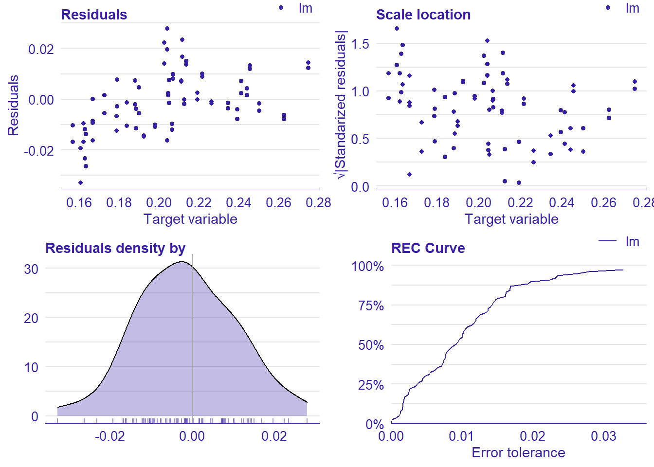
Figure 6: Manual Data fit with Regularized Regression and MARS, Year 2014 - 2018
## TableGrob (2 x 2) "arrange": 4 grobs
##   z     cells    name           grob
## 1 1 (1-1,1-1) arrange gtable[layout]
## 2 2 (1-1,2-2) arrange gtable[layout]
## 3 3 (2-2,1-1) arrange gtable[layout]
## 4 4 (2-2,2-2) arrange gtable[layout]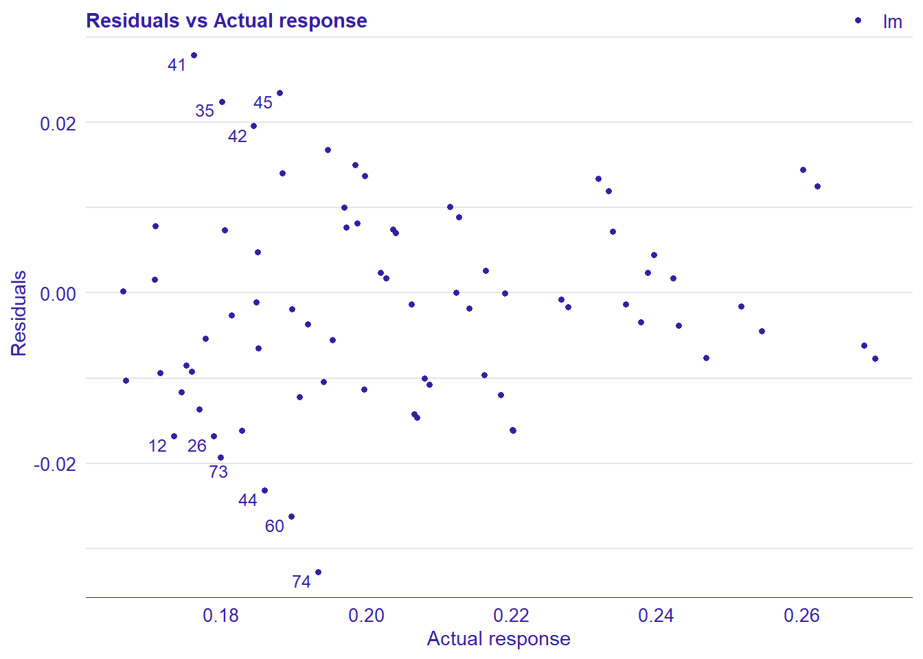
Figure 7: Manual Data fit with Regularized Regression and MARS, Year 2014 - 2018
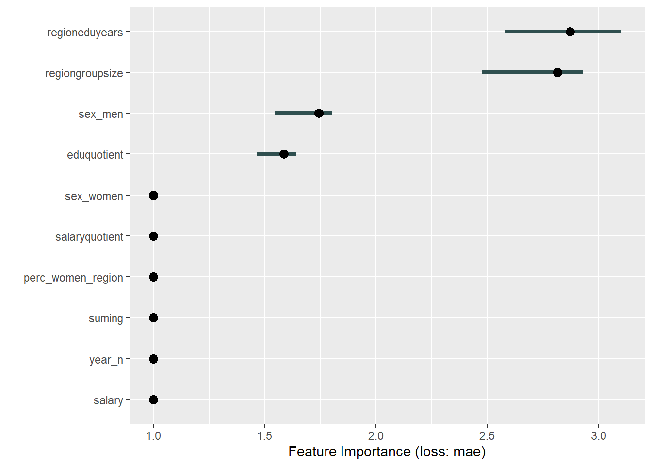
Figure 8: Manual Data fit with Regularized Regression and MARS, Year 2014 - 2018
##
## Attaching package: 'patchwork'
## The following object is masked from 'package:MASS':
##
## area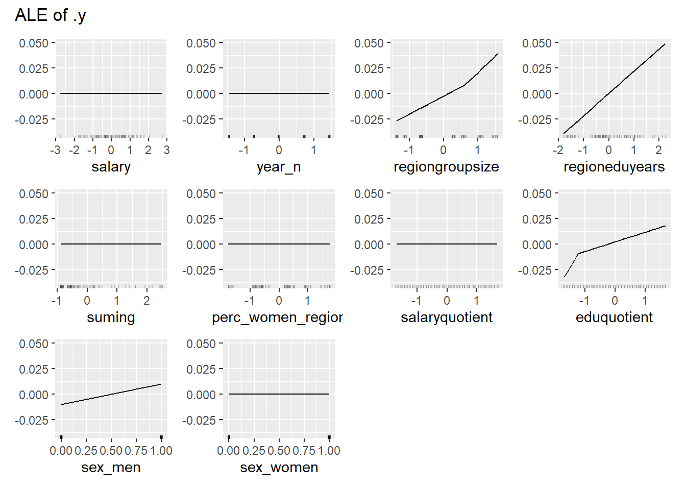
Figure 9: Manual Data fit with Regularized Regression and MARS, Year 2014 - 2018
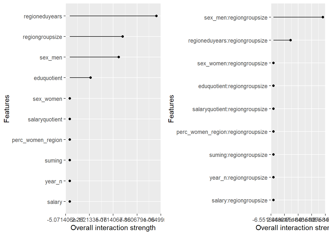
Figure 10: Manual Data fit with Regularized Regression and MARS, Year 2014 - 2018
## TableGrob (1 x 2) "arrange": 2 grobs
##   z     cells    name           grob
## 1 1 (1-1,1-1) arrange gtable[layout]
## 2 2 (1-1,2-2) arrange gtable[layout]
Data fit with Regularized Regression
X <- model.matrix(perc_women_eng_region ~ ., tbnum)[, -1]

Y <- tbnum$perc_women_eng_region

set.seed(123)  # for reproducibility
model <- caret::train(
    x = X,
    y = Y,
    weights = tbnum_weights,
    method = "glmnet",
    preProc = c("zv", "center", "scale"),
    trControl = trainControl(method = "cv", number = 10),
    tuneLength = 20
)
## Warning in nominalTrainWorkflow(x = x, y = y, wts = weights, info = trainInfo, :
## There were missing values in resampled performance measures.plot_model(model)##
## [1] "Model RMSE: 0.0115236920245644"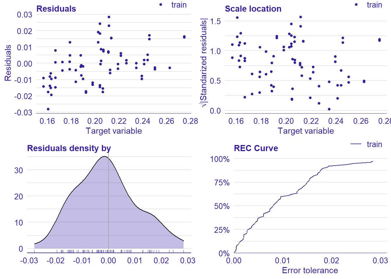
Figure 11: Data fit with Regularized Regression, Year 2014 - 2018
## TableGrob (2 x 2) "arrange": 4 grobs
##   z     cells    name           grob
## 1 1 (1-1,1-1) arrange gtable[layout]
## 2 2 (1-1,2-2) arrange gtable[layout]
## 3 3 (2-2,1-1) arrange gtable[layout]
## 4 4 (2-2,2-2) arrange gtable[layout]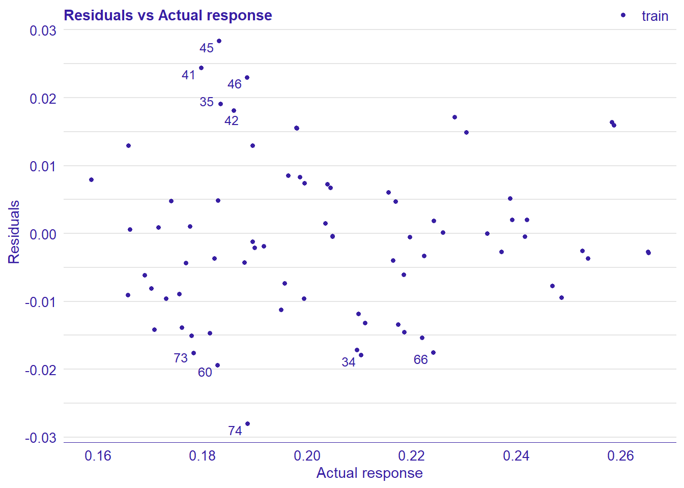
Figure 12: Data fit with Regularized Regression, Year 2014 - 2018
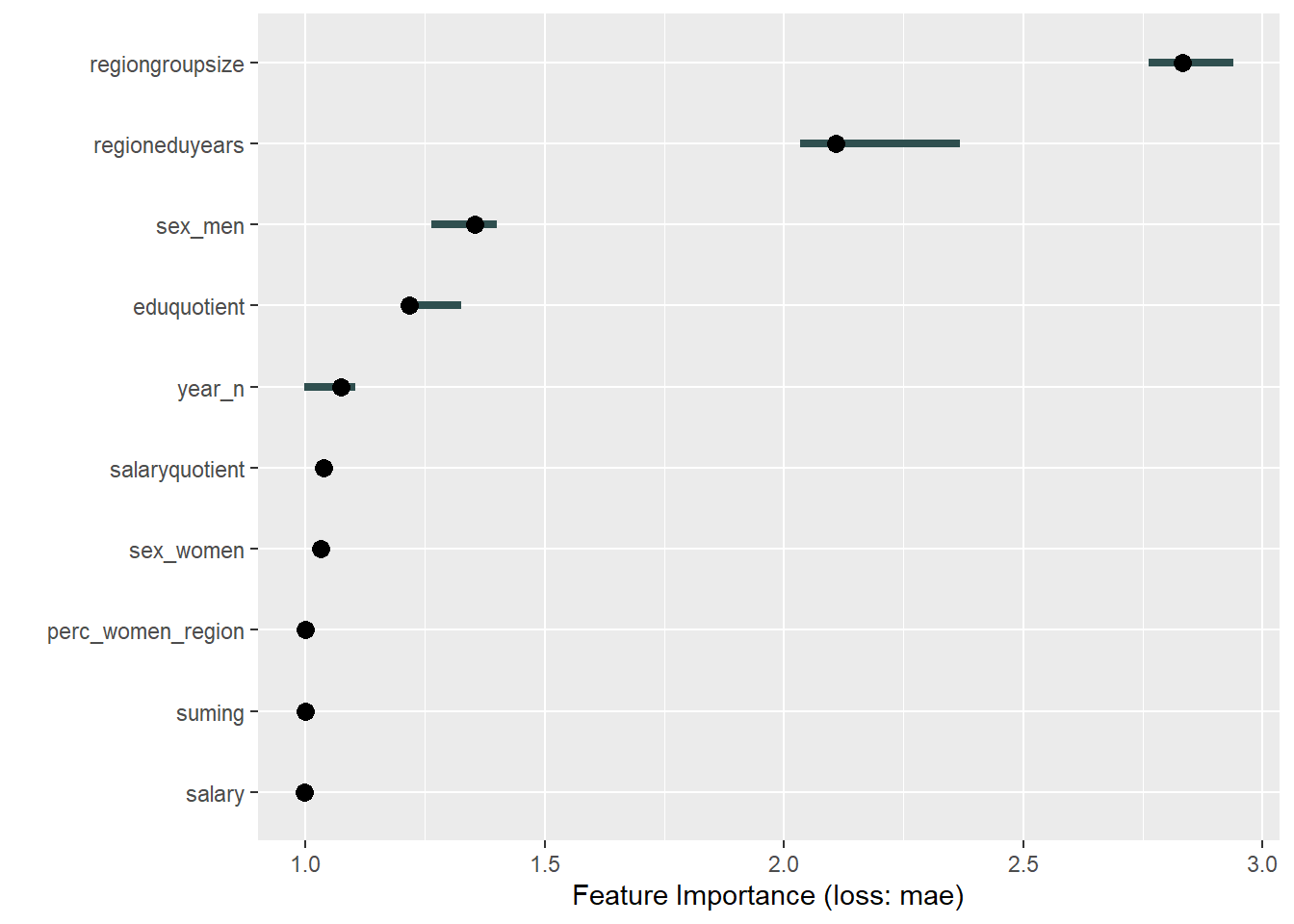
Figure 13: Data fit with Regularized Regression, Year 2014 - 2018
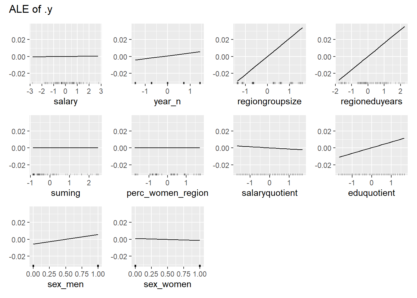
Figure 14: Data fit with Regularized Regression, Year 2014 - 2018
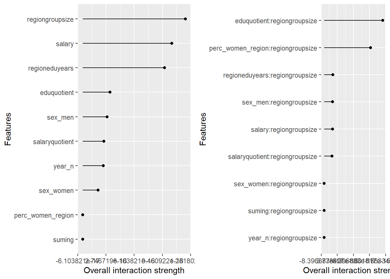
Figure 15: Data fit with Regularized Regression, Year 2014 - 2018
## TableGrob (1 x 2) "arrange": 2 grobs
##   z     cells    name           grob
## 1 1 (1-1,1-1) arrange gtable[layout]
## 2 2 (1-1,2-2) arrange gtable[layout]
Data fit with Multivariate Adaptive Regression Splines
hyper_grid <- expand.grid(
  degree = 1,
  nprune = seq(2, 100, length.out = 10) %>% floor()
)

set.seed(123)  # for reproducibility
model <- caret::train(
  x = data.frame(subset(tbnum, select = -perc_women_eng_region)),
  y = tbnum$perc_women_eng_region,
  method = "earth",
  weights = tbnum_weights,
  trControl = trainControl(method = "cv", number = 10),
  tuneGrid = hyper_grid
)

plot_model(model)
## Warning in if (class(response) == "data.frame") response <- as.matrix(response):
## the condition has length > 1 and only the first element will be used
## Warning in if (class(response) == "data.frame") response <- as.matrix(response):
## the condition has length > 1 and only the first element will be used##
## [1] "Model RMSE: 0.00915463662070812"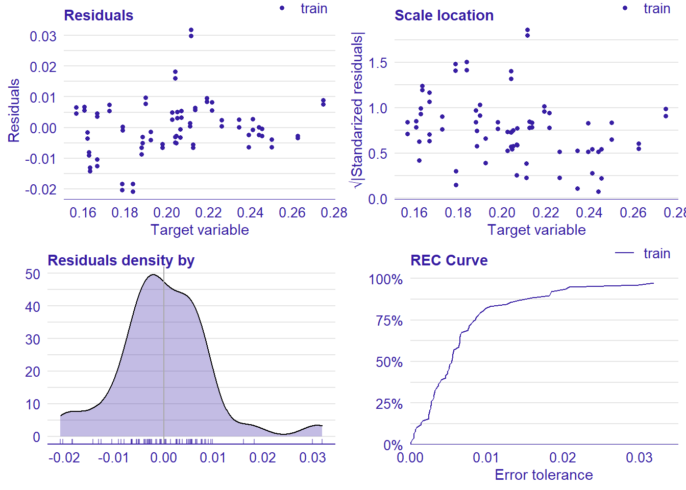
Figure 16: Data fit with Multivariate Adaptive Regression Splines, Year 2014 - 2018
## TableGrob (2 x 2) "arrange": 4 grobs
##   z     cells    name           grob
## 1 1 (1-1,1-1) arrange gtable[layout]
## 2 2 (1-1,2-2) arrange gtable[layout]
## 3 3 (2-2,1-1) arrange gtable[layout]
## 4 4 (2-2,2-2) arrange gtable[layout]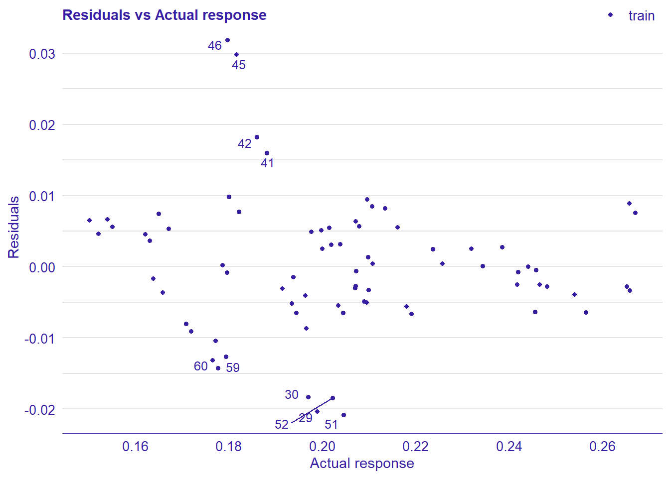
Figure 17: Data fit with Multivariate Adaptive Regression Splines, Year 2014 - 2018
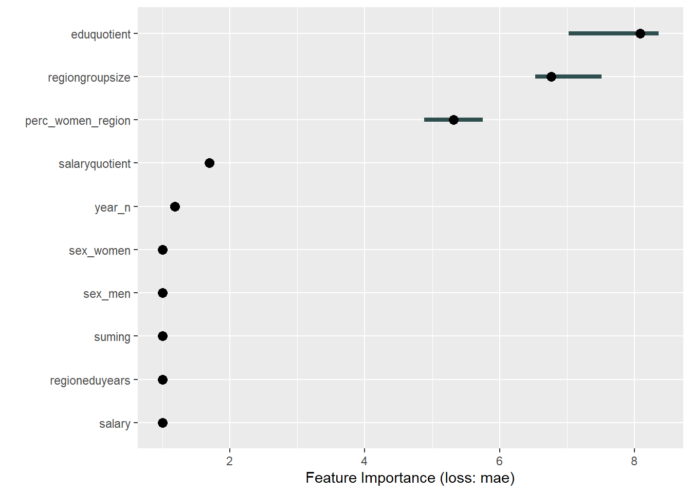
Figure 18: Data fit with Multivariate Adaptive Regression Splines, Year 2014 - 2018
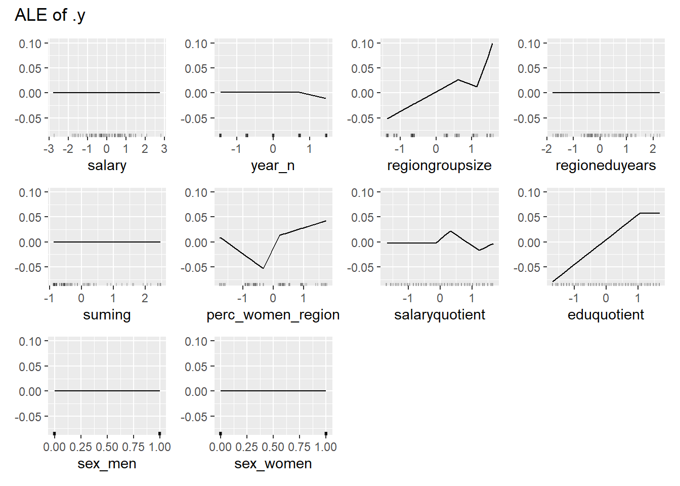
Figure 19: Data fit with Multivariate Adaptive Regression Splines, Year 2014 - 2018
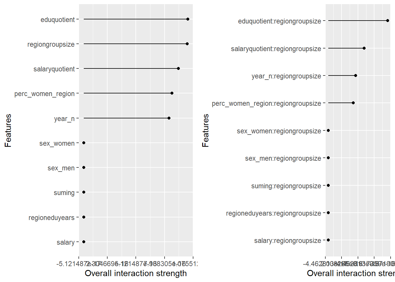
Figure 20: Data fit with Multivariate Adaptive Regression Splines, Year 2014 - 2018
## TableGrob (1 x 2) "arrange": 2 grobs
##   z     cells    name           grob
## 1 1 (1-1,1-1) arrange gtable[layout]
## 2 2 (1-1,2-2) arrange gtable[layout]
Data fit with decision tree bag
set.seed(123)
model <- caret::train(
  perc_women_eng_region ~ .,
  data = tbnum,
  method = "treebag",
  weights = tbnum_weights,
  trControl = trainControl(method = "cv", number = 10),
  nbagg = 50,
  control = rpart.control(minsplit = 2, cp = 0)
)

plot_model(model)
##
## [1] "Model RMSE: 0.00341044239371977"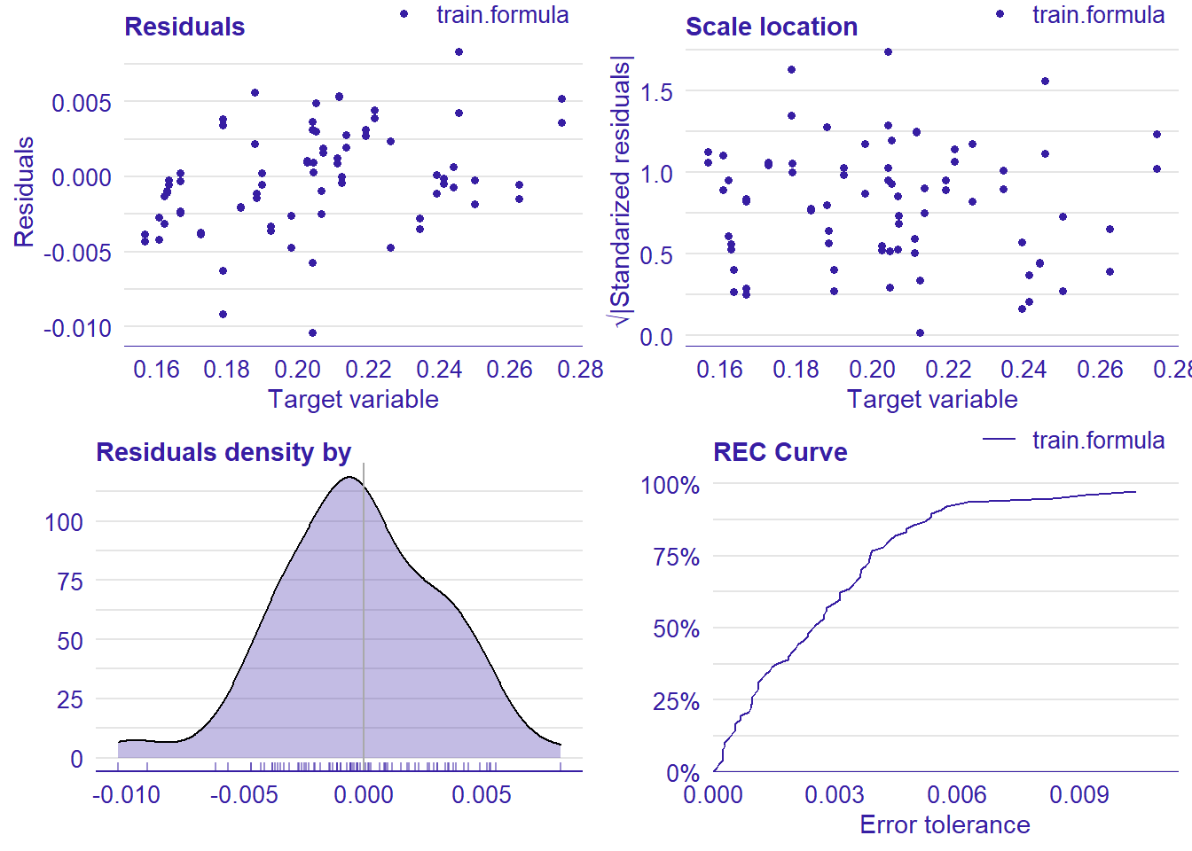
Figure 21: Data fit with decision tree bag, Year 2014 - 2018
## TableGrob (2 x 2) "arrange": 4 grobs
##   z     cells    name           grob
## 1 1 (1-1,1-1) arrange gtable[layout]
## 2 2 (1-1,2-2) arrange gtable[layout]
## 3 3 (2-2,1-1) arrange gtable[layout]
## 4 4 (2-2,2-2) arrange gtable[layout]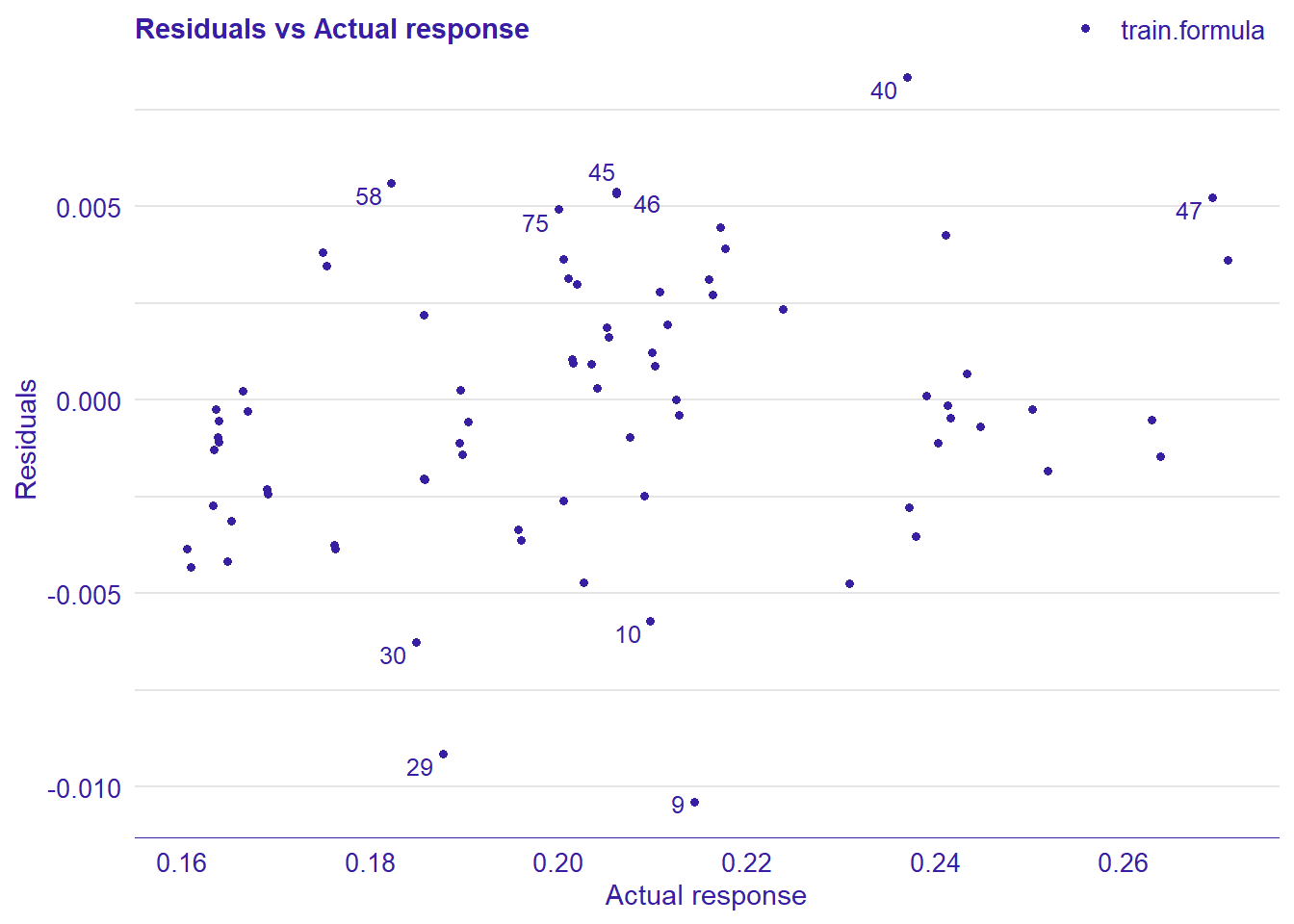
Figure 22: Data fit with decision tree bag, Year 2014 - 2018
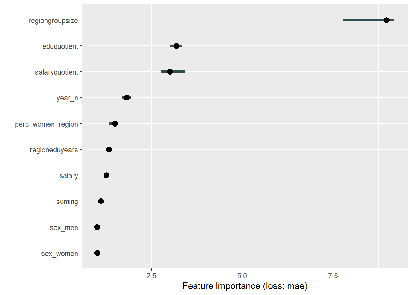
Figure 23: Data fit with decision tree bag, Year 2014 - 2018
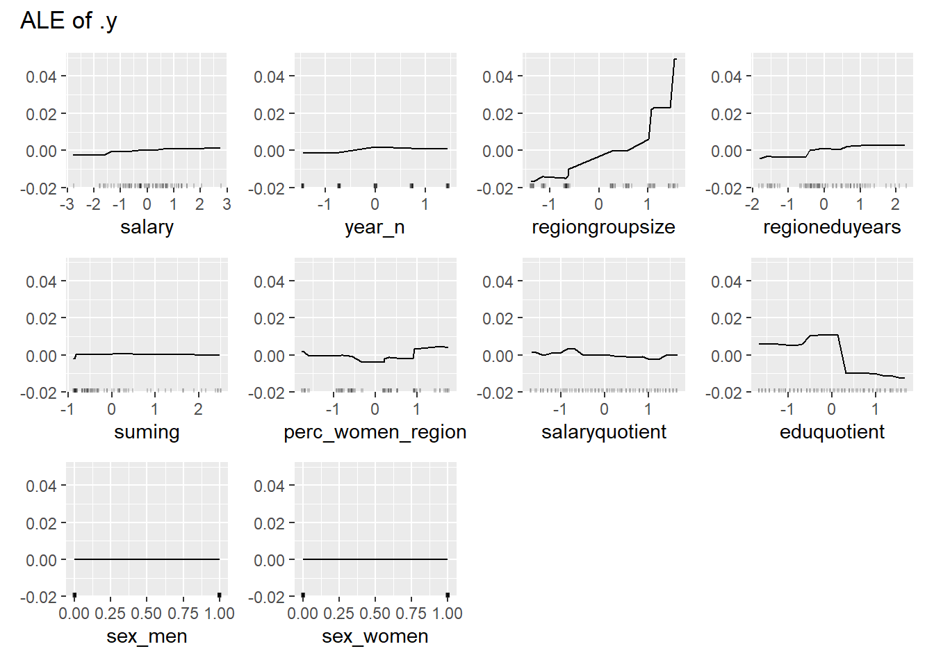
Figure 24: Data fit with decision tree bag, Year 2014 - 2018
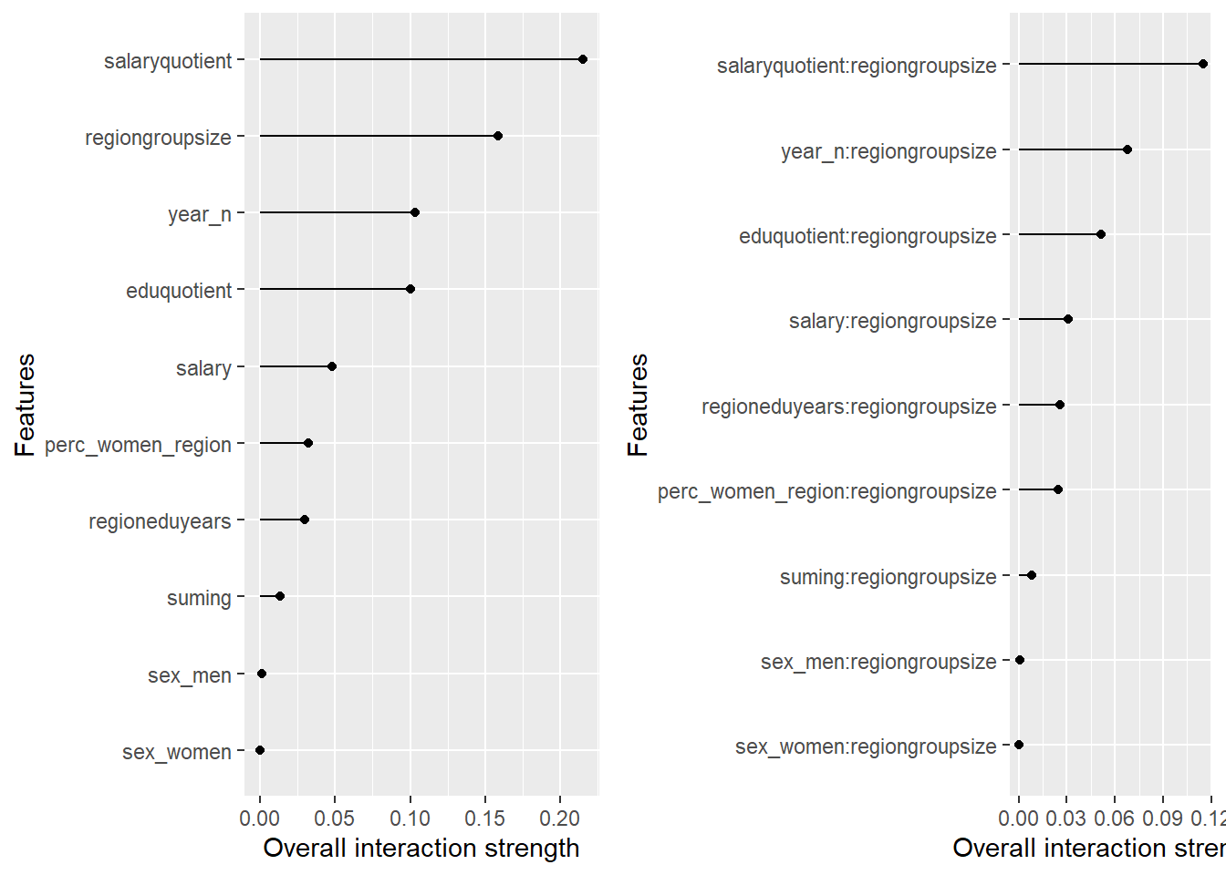
Figure 25: Data fit with decision tree bag, Year 2014 - 2018
## TableGrob (1 x 2) "arrange": 2 grobs
##   z     cells    name           grob
## 1 1 (1-1,1-1) arrange gtable[layout]
## 2 2 (1-1,2-2) arrange gtable[layout]
Data fit with Random Forest
set.seed(123)
invisible(capture.output(model <- caret::train(
   perc_women_eng_region  ~ .,
   data = tbnum,
   weights = tbnum_weights,
   method = "ranger",
   trControl = trainControl(method = "cv", number = 5, verboseIter = T, classProbs = T),
   num.trees = 100,
   importance = "permutation")))
## Warning in train.default(x, y, weights = w, ...): cannnot compute class
## probabilities for regressionplot_model(model)##
## [1] "Model RMSE: 0.00876237694751394"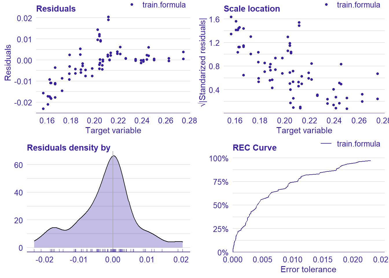
Figure 26: Data fit with Random Forest, Year 2014 - 2018
## TableGrob (2 x 2) "arrange": 4 grobs
##   z     cells    name           grob
## 1 1 (1-1,1-1) arrange gtable[layout]
## 2 2 (1-1,2-2) arrange gtable[layout]
## 3 3 (2-2,1-1) arrange gtable[layout]
## 4 4 (2-2,2-2) arrange gtable[layout]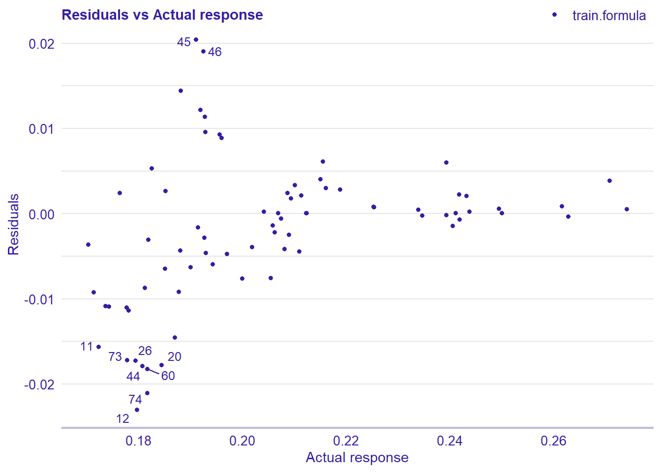
Figure 27: Data fit with Random Forest, Year 2014 - 2018
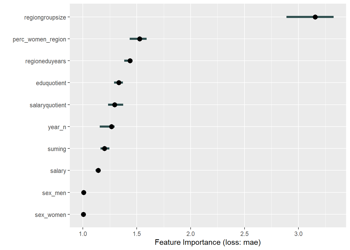
Figure 28: Data fit with Random Forest, Year 2014 - 2018
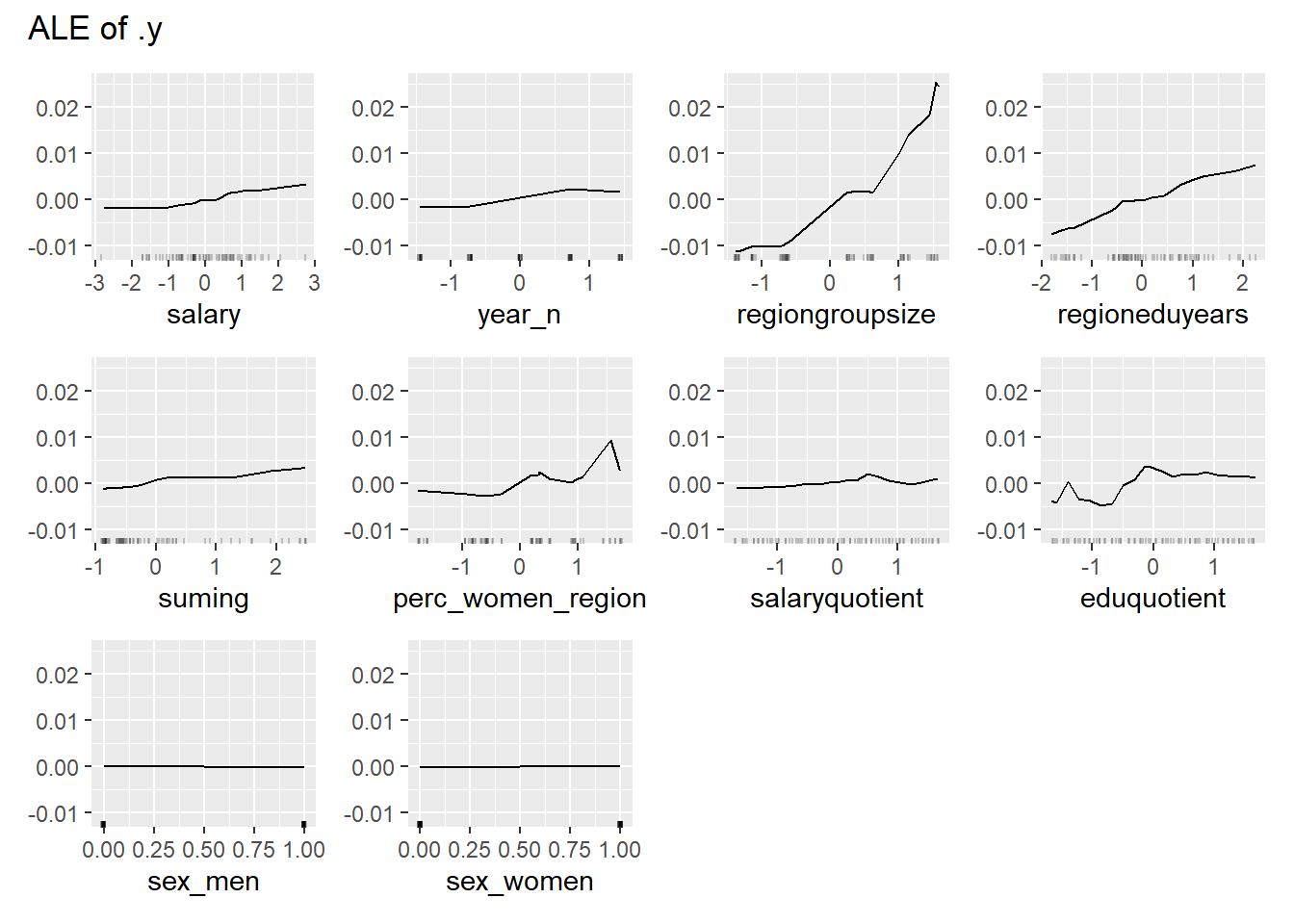
Figure 29: Data fit with Random Forest, Year 2014 - 2018
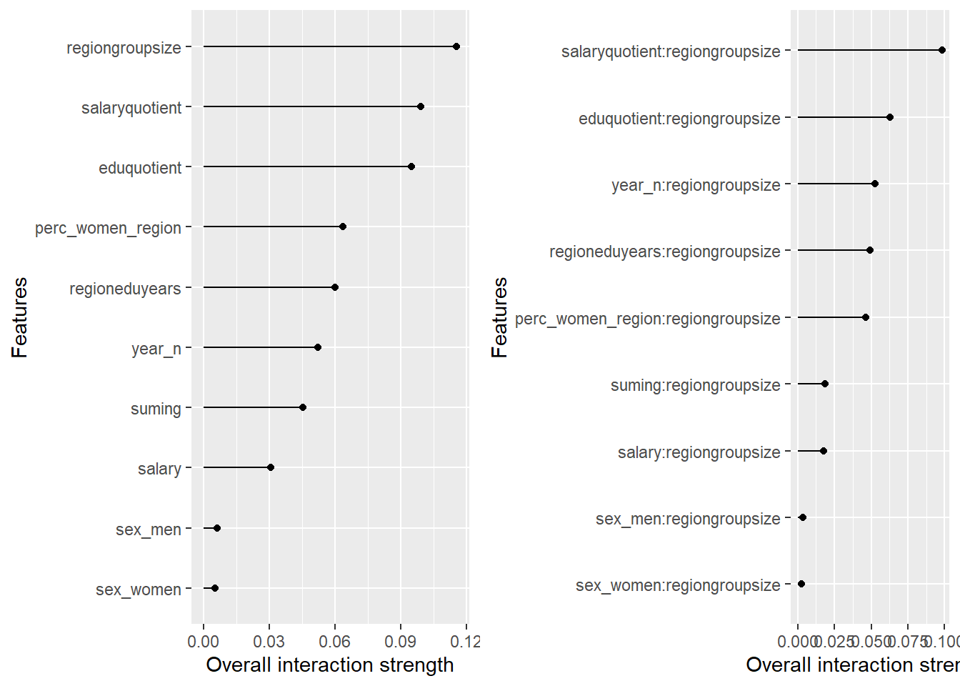
Figure 30: Data fit with Random Forest, Year 2014 - 2018
## TableGrob (1 x 2) "arrange": 2 grobs
##   z     cells    name           grob
## 1 1 (1-1,1-1) arrange gtable[layout]
## 2 2 (1-1,2-2) arrange gtable[layout]
Data fit with Gradient Boosting Machine
tr <- trainControl(method = "repeatedcv", number = 10, repeats = 5)

tg <- expand.grid(shrinkage = seq(0.1),
   interaction.depth = c(3),
   n.minobsinnode = c(10),
   n.trees = c(100))

set.seed(123)
model <- caret::train(
   perc_women_eng_region ~ .,
   data = tbnum,
   weights = tbnum_weights,
   method = "gbm",
   trControl = tr,
   tuneGrid = tg,
   verbose = FALSE)

plot_model(model)
##
## [1] "Model RMSE: 0.00352511569538881"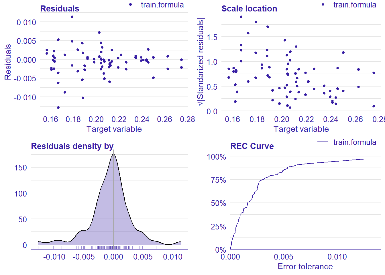
Figure 31: Data fit with Gradient Boosting Machine, Year 2014 - 2018
## TableGrob (2 x 2) "arrange": 4 grobs
##   z     cells    name           grob
## 1 1 (1-1,1-1) arrange gtable[layout]
## 2 2 (1-1,2-2) arrange gtable[layout]
## 3 3 (2-2,1-1) arrange gtable[layout]
## 4 4 (2-2,2-2) arrange gtable[layout]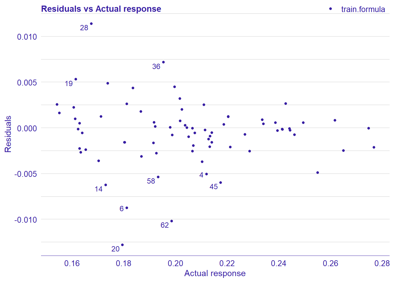
Figure 32: Data fit with Gradient Boosting Machine, Year 2014 - 2018
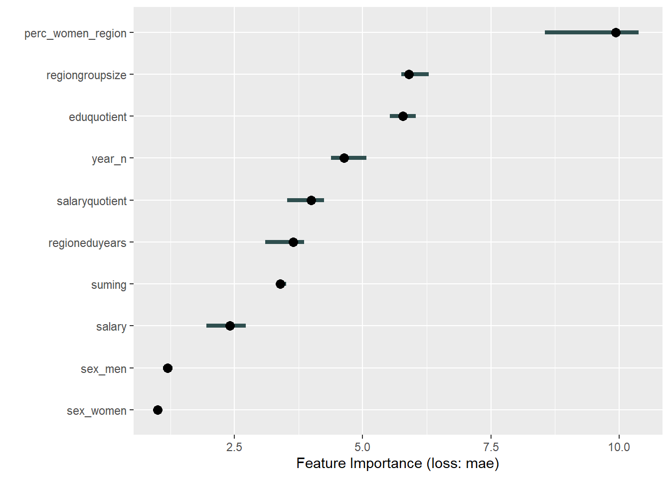
Figure 33: Data fit with Gradient Boosting Machine, Year 2014 - 2018
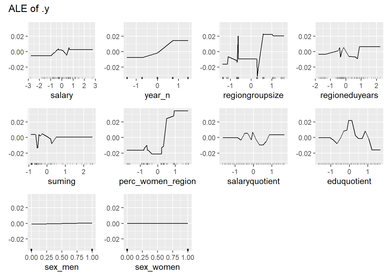
Figure 34: Data fit with Gradient Boosting Machine, Year 2014 - 2018
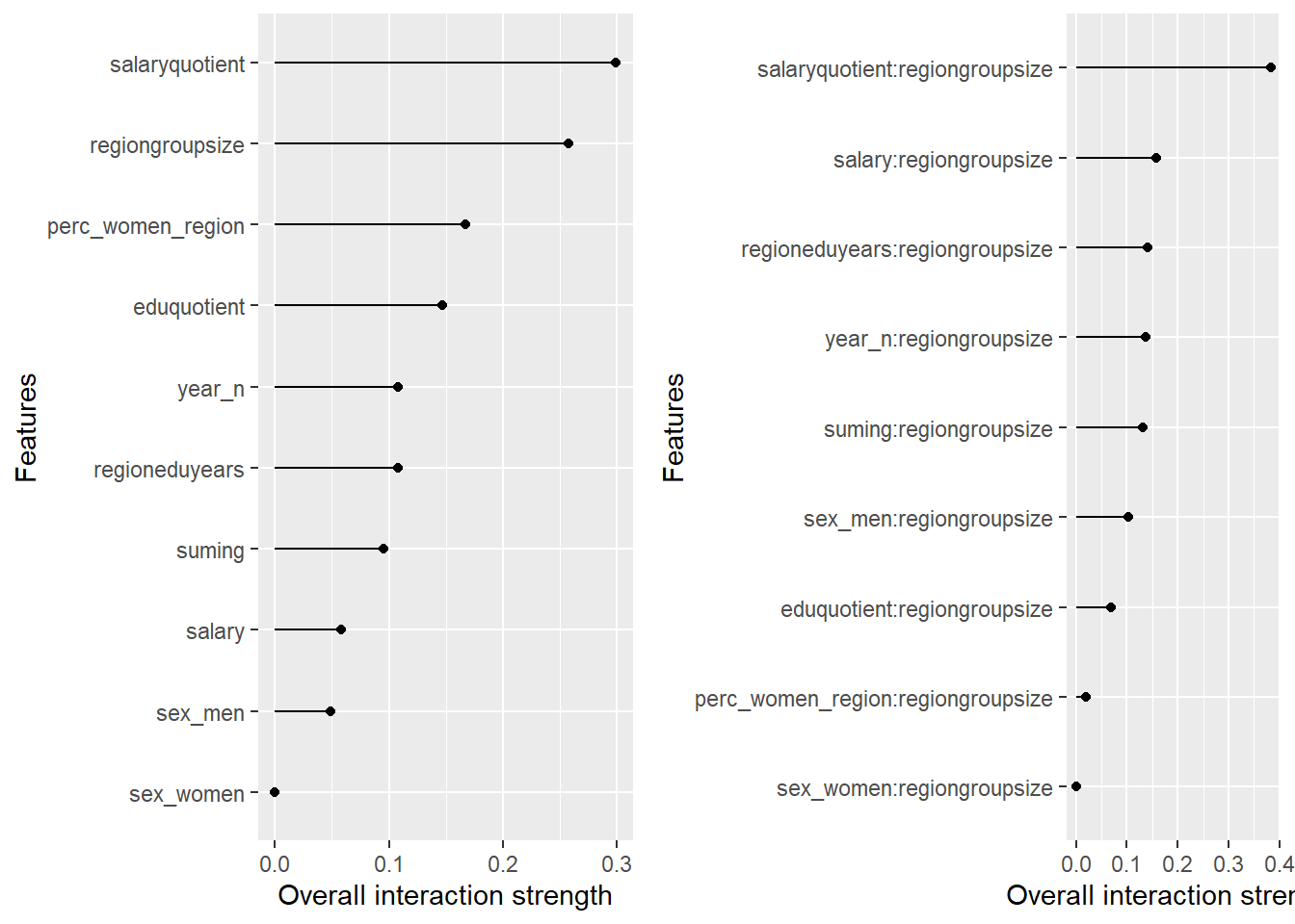
Figure 35: Data fit with Gradient Boosting Machine, Year 2014 - 2018
## TableGrob (1 x 2) "arrange": 2 grobs
##   z     cells    name           grob
## 1 1 (1-1,1-1) arrange gtable[layout]
## 2 2 (1-1,2-2) arrange gtable[layout]
Data fit with Deep Learning
rctrl1 <- trainControl(method = "cv", number = 3, returnResamp = "all")

set.seed(123)  # for reproducibility
model <- caret::train(
   perc_women_eng_region ~ .,
   data = tbnum,
   weights = tbnum_weights,
   method = "neuralnet",
   trControl = rctrl1,
   tuneGrid = data.frame(layer1 = 2:20, layer2 = 2:20, layer3 = 2:20),
   rep = 3,
   threshold = 0.0001,
   preProc = c("center", "scale"))

plot_model(model)
##
## [1] "Model RMSE: 0.00924842751296535"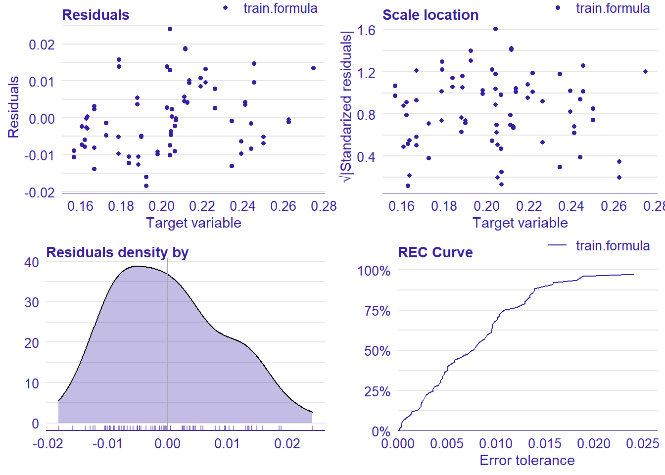
Figure 36: Data fit with Deep Learning, Year 2014 - 2018
## TableGrob (2 x 2) "arrange": 4 grobs
##   z     cells    name           grob
## 1 1 (1-1,1-1) arrange gtable[layout]
## 2 2 (1-1,2-2) arrange gtable[layout]
## 3 3 (2-2,1-1) arrange gtable[layout]
## 4 4 (2-2,2-2) arrange gtable[layout]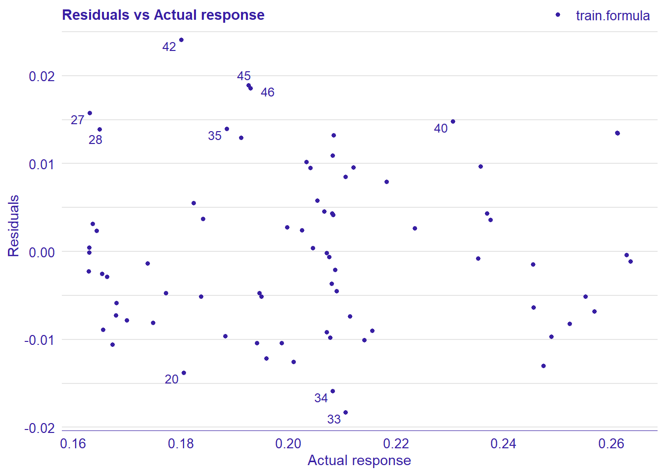
Figure 37: Data fit with Deep Learning, Year 2014 - 2018
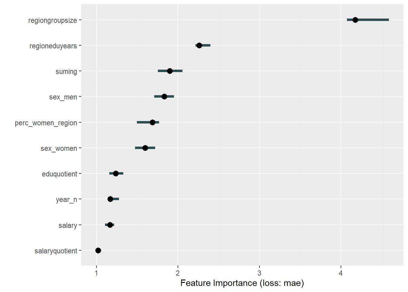
Figure 38: Data fit with Deep Learning, Year 2014 - 2018
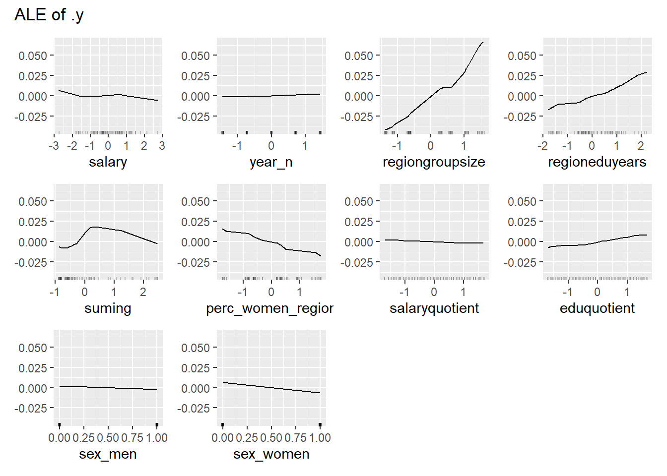
Figure 39: Data fit with Deep Learning, Year 2014 - 2018
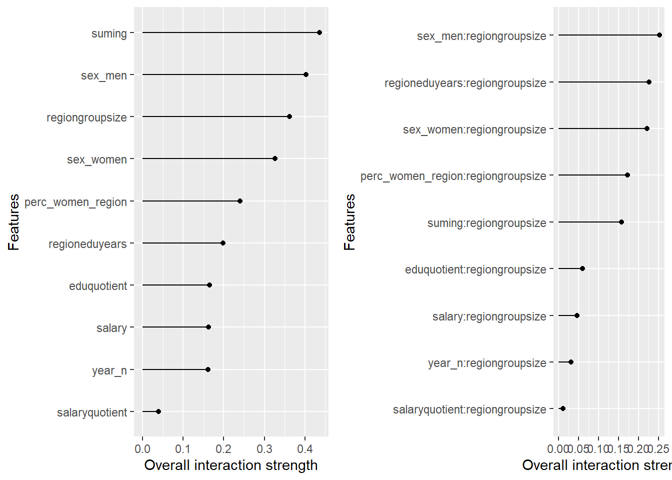
Figure 40: Data fit with Deep Learning, Year 2014 - 2018
## TableGrob (1 x 2) "arrange": 2 grobs
##   z     cells    name           grob
## 1 1 (1-1,1-1) arrange gtable[layout]
## 2 2 (1-1,2-2) arrange gtable[layout]
Data fit with Support Vector Machine
set.seed(123)  # for reproducibility
model <- caret::train(
  perc_women_eng_region ~ .,
  data = tbnum,
  weights = tbnum_weights,
  method = "svmRadial",
  preProcess = c("center", "scale"),
  trControl = trainControl(method = "cv", number = 10),
  tuneLength = 10
)

plot_model(model)
##
## [1] "Model RMSE: 0.00848330404577974"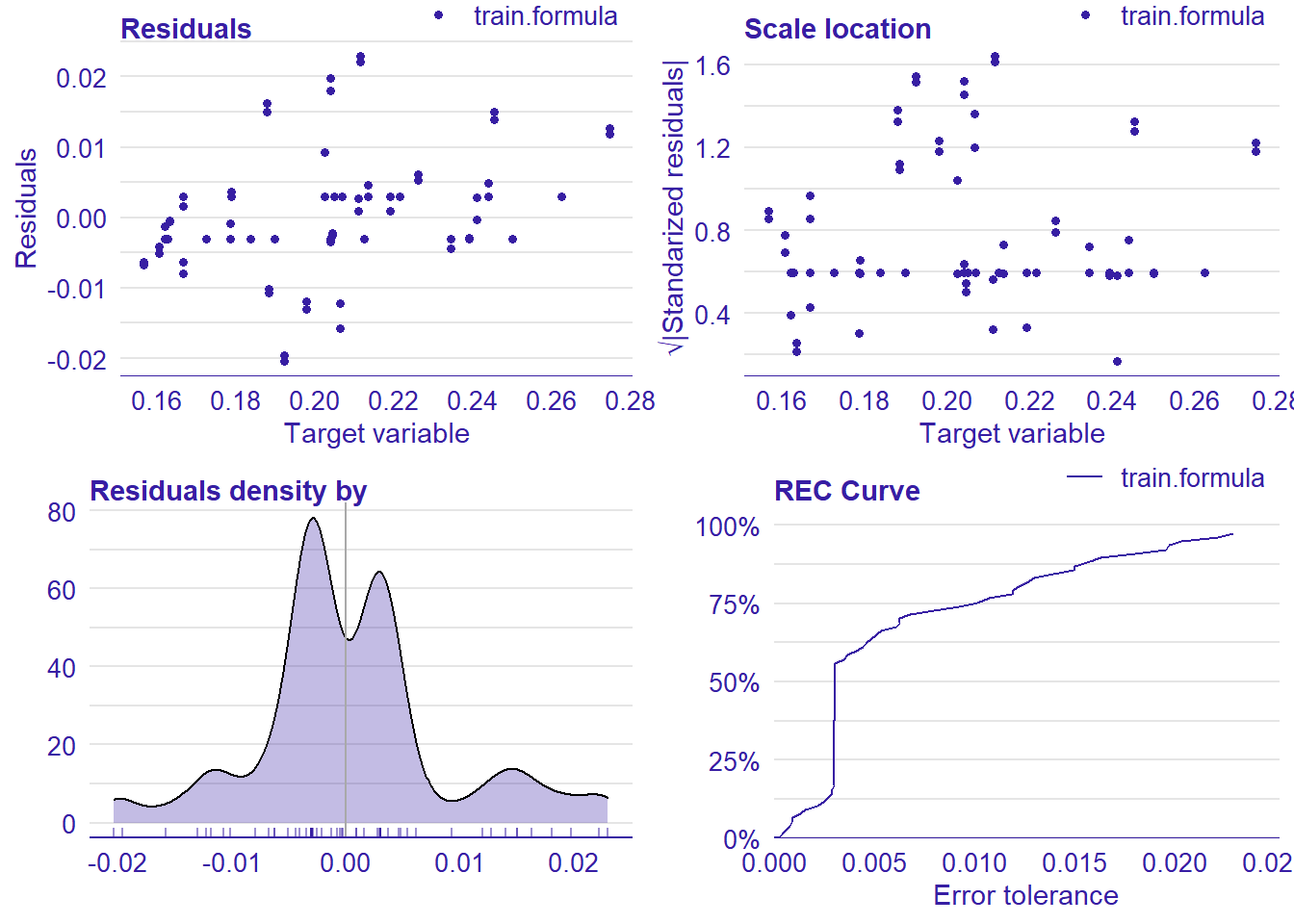
Figure 41: Data fit with Support Vector Machine, Year 2014 - 2018
## TableGrob (2 x 2) "arrange": 4 grobs
##   z     cells    name           grob
## 1 1 (1-1,1-1) arrange gtable[layout]
## 2 2 (1-1,2-2) arrange gtable[layout]
## 3 3 (2-2,1-1) arrange gtable[layout]
## 4 4 (2-2,2-2) arrange gtable[layout]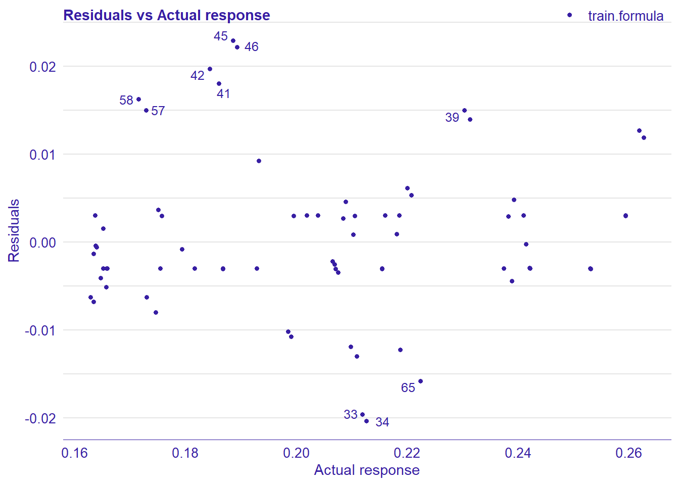
Figure 42: Data fit with Support Vector Machine, Year 2014 - 2018
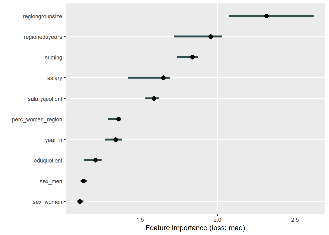
Figure 43: Data fit with Support Vector Machine, Year 2014 - 2018
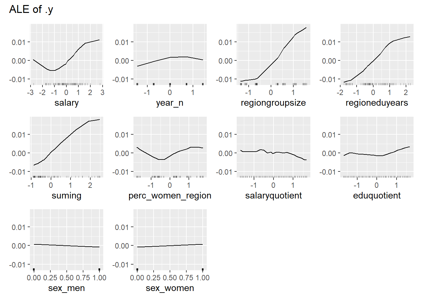
Figure 44: Data fit with Support Vector Machine, Year 2014 - 2018
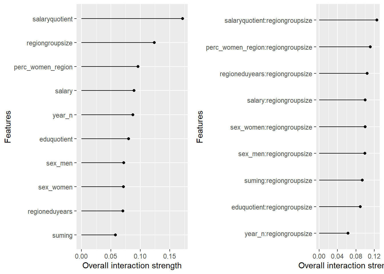
Figure 45: Data fit with Support Vector Machine, Year 2014 - 2018
## TableGrob (1 x 2) "arrange": 2 grobs
##   z     cells    name           grob
## 1 1 (1-1,1-1) arrange gtable[layout]
## 2 2 (1-1,2-2) arrange gtable[layout]