In a previous post, I analysed the feature importance for the per cent of engineers in Sweden who are women. I found that the size of the region is a feature that is significant for the per cent of engineers in Sweden who are women. In this post, I will analyse the feature importance of different occupational groups in Sweden. I will use an ensemble of linear models in my analysis.
Statistics Sweden use NUTS (Nomenclature des Unités Territoriales Statistiques), which is the EU’s hierarchical regional division, to specify the regions.
Please send suggestions for improvement of the analysis to ranalystatisticssweden@gmail.com.
First, define libraries and functions.
library (tidyverse)## -- Attaching packages -------------------------------------------------- tidyverse 1.3.0 --## v ggplot2 3.3.0 v purrr 0.3.4
## v tibble 3.0.0 v dplyr 0.8.5
## v tidyr 1.0.2 v stringr 1.4.0
## v readr 1.3.1 v forcats 0.5.0## -- Conflicts ----------------------------------------------------- tidyverse_conflicts() --
## x dplyr::filter() masks stats::filter()
## x dplyr::lag() masks stats::lag()library (broom)
library (car)## Loading required package: carData##
## Attaching package: 'car'## The following object is masked from 'package:dplyr':
##
## recode## The following object is masked from 'package:purrr':
##
## somelibrary (caret) ## Loading required package: lattice##
## Attaching package: 'caret'## The following object is masked from 'package:purrr':
##
## liftlibrary (recipes) ##
## Attaching package: 'recipes'## The following object is masked from 'package:stringr':
##
## fixed## The following object is masked from 'package:stats':
##
## steplibrary (PerformanceAnalytics)## Loading required package: xts## Loading required package: zoo##
## Attaching package: 'zoo'## The following objects are masked from 'package:base':
##
## as.Date, as.Date.numeric##
## Attaching package: 'xts'## The following objects are masked from 'package:dplyr':
##
## first, last##
## Attaching package: 'PerformanceAnalytics'## The following object is masked from 'package:graphics':
##
## legendlibrary (ggpubr)## Loading required package: magrittr##
## Attaching package: 'magrittr'## The following object is masked from 'package:purrr':
##
## set_names## The following object is masked from 'package:tidyr':
##
## extractlibrary (ipred)
library (iml)
library (SuperLearner)## Loading required package: nnls## Super Learner## Version: 2.0-26## Package created on 2019-10-27library (scatterplot3d)
readfile <- function (file1){read_csv (file1, col_types = cols(), locale = readr::locale (encoding = "latin1"), na = c("..", "NA")) %>%
gather (starts_with("19"), starts_with("20"), key = "year", value = groupsize) %>%
drop_na() %>%
mutate (year_n = parse_number (year))
}
perc_women <- function(x){
ifelse (length(x) == 2, x[2] / (x[1] + x[2]), NA)
}
nuts <- read.csv("nuts.csv") %>%
mutate(NUTS2_sh = substr(NUTS2, 3, 4))
nuts %>%
distinct (NUTS2_en) %>%
knitr::kable(
booktabs = TRUE,
caption = 'Nomenclature des Unités Territoriales Statistiques (NUTS)')| NUTS2_en |
|---|
| SE11 Stockholm |
| SE12 East-Central Sweden |
| SE21 Småland and islands |
| SE22 South Sweden |
| SE23 West Sweden |
| SE31 North-Central Sweden |
| SE32 Central Norrland |
| SE33 Upper Norrland |
SL.lm.caret <- function(..., method = "lm", tuneLength = 3, obsWeights = obsWeights, trControl = caret::trainControl(method = "cv", number = 10, verboseIter = FALSE)){
    suppressWarnings(SL.caret(..., obsWeights = obsWeights, method = method, tuneLength = tuneLength, trControl = trControl))
}

SL.lmStepAIC.caret <- function(..., method = "lmStepAIC", tuneLength = 3, obsWeights = obsWeights, trControl = caret::trainControl(method = "cv", number = 10, verboseIter = FALSE)){
    suppressWarnings(SL.caret(..., obsWeights = obsWeights, method = method, tuneLength = tuneLength, trControl = trControl))
}

SL.bayesglm.caret <- function(..., method = "bayesglm", tuneLength = 3, obsWeights = obsWeights, trControl = caret::trainControl(method = "cv", number = 10, verboseIter = FALSE)){
    suppressWarnings(SL.caret(..., obsWeights = obsWeights, method = method, tuneLength = tuneLength, trControl = trControl))
}

SL.rlm.caret <- function(..., method = "rlm", tuneLength = 3, obsWeights = obsWeights, trControl = caret::trainControl(method = "cv", number = 10, verboseIter = FALSE)){
    suppressWarnings(SL.caret(..., obsWeights = obsWeights, method = method, tuneLength = tuneLength, trControl = trControl))
}
The data tables are downloaded from Statistics Sweden. They are saved as a comma-delimited file without heading, UF0506A1.csv, http://www.statistikdatabasen.scb.se/pxweb/en/ssd/.
The tables:
UF0506A1_1.csv: Population 16-74 years of age by region, highest level of education, age and sex. Year 1985 - 2018 NUTS 2 level 2008- 10 year intervals (16-74)
000000CG_1: Average basic salary, monthly salary and women´s salary as a percentage of men´s salary by region, sector, occupational group (SSYK 2012) and sex. Year 2014 - 2018 Monthly salary All sectors.
000000CD_1.csv: Average basic salary, monthly salary and women´s salary as a percentage of men´s salary by region, sector, occupational group (SSYK 2012) and sex. Year 2014 - 2018 Number of employees All sectors.
The data is aggregated, the size of each group is in the column groupsize.
I have also included some calculated predictors from the original data.
perc_women: The percentage of women within each group defined by edulevel, region and year
perc_women_region: The percentage of women within each group defined by year and region
regioneduyears: The average number of education years per capita within each group defined by year and region
eduquotient: The quotient between regioneduyears for men and women
salaryquotient: The quotient between salary for men and women within each group defined by year and region
perc_women_eng_region: The percentage of women who are engineers within each group defined by year and region
numedulevel <- read.csv("edulevel_1.csv")

numedulevel[, 2] <- data.frame(c(8, 9, 10, 12, 13, 15, 22, NA))

tb <- readfile("000000CG_1.csv")
tb <- readfile("000000CD_1.csv") %>%
  left_join(tb, by = c("region", "year", "sex", "sector","occuptional  (SSYK 2012)"))

tb <- readfile("UF0506A1_1.csv") %>%
  right_join(tb, by = c("region", "year", "sex")) %>%
  right_join(numedulevel, by = c("level of education" = "level.of.education")) %>%
  filter(!is.na(eduyears)) %>%
  mutate(edulevel = `level of education`) %>%
  group_by(edulevel, region, year, sex, `occuptional  (SSYK 2012)`) %>%
  mutate(groupsize_all_ages = sum(groupsize)) %>%
  group_by(edulevel, region, year, `occuptional  (SSYK 2012)`) %>%
  mutate (perc_women = perc_women (groupsize_all_ages[1:2])) %>%
  mutate (suming = sum(groupsize.x)) %>%
  mutate (salary = (groupsize.y[2] * groupsize.x[2] + groupsize.y[1] * groupsize.x[1])/(groupsize.x[2] + groupsize.x[1])) %>%
  group_by (sex, year, region, `occuptional  (SSYK 2012)`) %>%
  mutate(regioneduyears_sex = sum(groupsize * eduyears) / sum(groupsize)) %>%
  mutate(regiongroupsize = sum(groupsize)) %>%
  mutate(suming_sex = groupsize.x) %>%
  group_by(region, year, `occuptional  (SSYK 2012)`) %>%
  mutate (sum_pop = sum(groupsize)) %>%
  mutate (regioneduyears = sum(groupsize * eduyears) / sum(groupsize)) %>%
  mutate (perc_women_region = perc_women (regiongroupsize[1:2])) %>%
  mutate (eduquotient = regioneduyears_sex[2] / regioneduyears_sex[1]) %>%
  mutate (salary_sex = groupsize.y) %>%
  mutate (salaryquotient = salary_sex[2] / salary_sex[1]) %>%
  mutate (perc_women_eng_region = perc_women(suming_sex[1:2])) %>%
  left_join(nuts %>% distinct (NUTS2_en, NUTS2_sh), by = c("region" = "NUTS2_en")) %>%
  drop_na()

summary(tb)
## region age level of education sex
## Length:29050 Length:29050 Length:29050 Length:29050
## Class :character Class :character Class :character Class :character
## Mode :character Mode :character Mode :character Mode :character
##
##
##
## year groupsize year_n sector
## Length:29050 Min. : 405 Min. :2014 Length:29050
## Class :character 1st Qu.: 25412 1st Qu.:2015 Class :character
## Mode :character Median : 61291 Median :2016 Mode :character
## Mean : 71345 Mean :2016
## 3rd Qu.:113524 3rd Qu.:2017
## Max. :271889 Max. :2018
## occuptional (SSYK 2012) groupsize.x year_n.x groupsize.y
## Length:29050 Min. : 100 Min. :2014 Min. : 20200
## Class :character 1st Qu.: 490 1st Qu.:2015 1st Qu.: 28900
## Mode :character Median : 1300 Median :2016 Median : 33900
## Mean : 3258 Mean :2016 Mean : 37066
## 3rd Qu.: 3400 3rd Qu.:2017 3rd Qu.: 42100
## Max. :45000 Max. :2018 Max. :133600
## year_n.y eduyears edulevel groupsize_all_ages
## Min. :2014 Min. : 8.00 Length:29050 Min. : 405
## 1st Qu.:2015 1st Qu.: 9.00 Class :character 1st Qu.: 25412
## Median :2016 Median :12.00 Mode :character Median : 61291
## Mean :2016 Mean :12.71 Mean : 71345
## 3rd Qu.:2017 3rd Qu.:15.00 3rd Qu.:113524
## Max. :2018 Max. :22.00 Max. :271889
## perc_women suming salary regioneduyears_sex
## Min. :0.3575 Min. : 240 Min. : 20661 Min. :11.18
## 1st Qu.:0.4343 1st Qu.: 1330 1st Qu.: 29046 1st Qu.:11.63
## Median :0.4655 Median : 3100 Median : 34041 Median :11.78
## Mean :0.4775 Mean : 6515 Mean : 37105 Mean :11.83
## 3rd Qu.:0.5132 3rd Qu.: 7400 3rd Qu.: 42068 3rd Qu.:12.09
## Max. :0.6423 Max. :60000 Max. :113976 Max. :12.55
## regiongroupsize suming_sex sum_pop regioneduyears
## Min. :128262 Min. : 100 Min. : 262870 Min. :11.39
## 1st Qu.:292864 1st Qu.: 490 1st Qu.: 596546 1st Qu.:11.56
## Median :528643 Median : 1300 Median :1057419 Median :11.82
## Mean :499413 Mean : 3258 Mean : 998826 Mean :11.83
## 3rd Qu.:708813 3rd Qu.: 3400 3rd Qu.:1417931 3rd Qu.:11.93
## Max. :827940 Max. :45000 Max. :1655215 Max. :12.41
## perc_women_region eduquotient salary_sex salaryquotient
## Min. :0.4831 Min. :1.019 Min. : 20200 Min. :0.6423
## 1st Qu.:0.4890 1st Qu.:1.027 1st Qu.: 28900 1st Qu.:0.9144
## Median :0.4937 Median :1.032 Median : 33900 Median :0.9556
## Mean :0.4931 Mean :1.033 Mean : 37066 Mean :0.9502
## 3rd Qu.:0.4971 3rd Qu.:1.040 3rd Qu.: 42100 3rd Qu.:0.9941
## Max. :0.5014 Max. :1.047 Max. :133600 Max. :1.3090
## perc_women_eng_region NUTS2_sh
## Min. :0.01659 Length:29050
## 1st Qu.:0.30876 Class :character
## Median :0.56000 Mode :character
## Mean :0.52565
## 3rd Qu.:0.72414
## Max. :0.94527tbtemp <- ungroup(tb) %>% dplyr::select(salary, suming, year_n, sum_pop, regioneduyears, perc_women_region, salaryquotient, eduquotient, perc_women_eng_region, `occuptional (SSYK 2012)`)
tb_unique <- unique(tbtemp)I will use SuperLearner to train the ensemble consisting of four linear models without interactions. The four models are Linear Regression (lm), Linear Regression with Stepwise Selection (lmStepAIC), Bayesian Generalized Linear Model (bayesglm) and Robust Linear Model (rlm).
summary_table = vector()
cor_table = vector()
sp_table <- vector()
rmse_table <- vector()

for (i in unique(tb_unique$`occuptional  (SSYK 2012)`)){
  temp <- filter(tb_unique, `occuptional  (SSYK 2012)` == i)
  if (dim(temp)[1] > 20){
     temp_weights = temp$suming
     temp <- dplyr::select(temp, - c(`occuptional  (SSYK 2012)`, suming))
     blueprint <- recipe(perc_women_eng_region ~ ., data = temp) %>%
       step_integer(matches("Qual|Cond|QC|Qu")) %>%
       step_center(all_numeric(), -all_outcomes()) %>%
       step_scale(all_numeric(), -all_outcomes()) %>%
       step_dummy(all_nominal(), -all_outcomes(), one_hot = TRUE)
     prepare <- prep(blueprint, training = temp)
     temp <- bake(prepare, new_data = temp)

     invisible(capture.output(model <- SuperLearner(
        temp$perc_women_eng_region,
        data.frame(dplyr::select(temp, -c(perc_women_eng_region))),
        family = gaussian(),
        verbose = FALSE,
        obsWeights = temp_weights,
        SL.library = list("SL.lm.caret", "SL.lmStepAIC.caret", "SL.bayesglm.caret", "SL.rlm.caret"))))

     pred <- function(object, newdata){
       predict(model, newdata=newdata, onlySL = TRUE)$pred
     }

     predictor <- Predictor$new(model,
        data = dplyr::select(temp, -perc_women_eng_region),
        y = temp$perc_women_eng_region,
        predict.fun = pred)

     imp <- FeatureImp$new(predictor, loss = "mae", n.repetitions = 30)

     summary_table <- rbind(summary_table, mutate(tibble(.rows = 7), importance = imp$results$importance, feature = imp$results$feature, importance.05 = imp$results$importance.05, ssyk = i))

     cor_table <- rbind(cor_table, mutate(tibble(.rows = 7), feature = colnames(dplyr::select(temp, -c(perc_women_eng_region))), cor = cor(dplyr::select(temp, -c(perc_women_eng_region)), temp$perc_women_eng_region), ssyk = i))

     sp_table <- rbind(sp_table, mutate(tibble(.rows = 4), coef = model$coef, model = names(model$coef),  ssyk = i))

     prs <- postResample(pred = predict(model)$pred, obs = temp$perc_women_eng_region)

     rmse_table <- rbind(rmse_table, mutate(tibble(.rows = 1), RMSE = prs[1], Rsquared = prs[2], MAE = prs[3], ssyk = i))
  }
}
## Registered S3 methods overwritten by 'lme4':
## method from
## cooks.distance.influence.merMod car
## influence.merMod car
## dfbeta.influence.merMod car
## dfbetas.influence.merMod carThe table below shows the feature values for the different occupation groups and if there is a single important feature (diff1) or if there are two important features (diff2) for the occupational group. The Rsquared value shows if the model for the occupational group does have a good fit.
summary_table %>%
  group_by(ssyk) %>%
  group_by(ssyk) %>%
  dplyr::mutate(diff1 = importance.05[1] / importance[2]) %>%
  dplyr::mutate(diff2 = importance.05[2] / importance[3]) %>%
  left_join(cor_table, by = c("ssyk", "feature")) %>%
  left_join(sp_table %>% spread(model, coef), by=c("ssyk")) %>%
  left_join(rmse_table, by=c("ssyk")) %>%
  dplyr::select(ssyk, feature, importance, importance.05, diff1, diff2, Rsquared) %>%
  knitr::kable(
     booktabs = TRUE,
caption = 'Feature values for different occupation groups')| ssyk | feature | importance | importance.05 | diff1 | diff2 | Rsquared |
|---|---|---|---|---|---|---|
| 123 Administration and planning managers | eduquotient | 3.8170179 | 3.2624044 | 0.9992710 | 0.9746650 | 0.5296568 |
| 123 Administration and planning managers | sum_pop | 3.2647844 | 2.6462447 | 0.9992710 | 0.9746650 | 0.5296568 |
| 123 Administration and planning managers | salary | 2.7150299 | 2.3345443 | 0.9992710 | 0.9746650 | 0.5296568 |
| 123 Administration and planning managers | regioneduyears | 2.5260824 | 2.1015060 | 0.9992710 | 0.9746650 | 0.5296568 |
| 123 Administration and planning managers | salaryquotient | 1.2063518 | 1.0434914 | 0.9992710 | 0.9746650 | 0.5296568 |
| 123 Administration and planning managers | perc_women_region | 1.1813452 | 1.0858792 | 0.9992710 | 0.9746650 | 0.5296568 |
| 123 Administration and planning managers | year_n | 1.0740710 | 1.0155535 | 0.9992710 | 0.9746650 | 0.5296568 |
| 141 Primary and secondary schools and adult education managers | regioneduyears | 2.7494050 | 2.2970027 | 1.3327022 | 0.9503406 | 0.6950328 |
| 141 Primary and secondary schools and adult education managers | year_n | 1.7235678 | 1.4984603 | 1.3327022 | 0.9503406 | 0.6950328 |
| 141 Primary and secondary schools and adult education managers | salary | 1.5767613 | 1.4698417 | 1.3327022 | 0.9503406 | 0.6950328 |
| 141 Primary and secondary schools and adult education managers | sum_pop | 1.0000000 | 1.0000000 | 1.3327022 | 0.9503406 | 0.6950328 |
| 141 Primary and secondary schools and adult education managers | perc_women_region | 1.0000000 | 1.0000000 | 1.3327022 | 0.9503406 | 0.6950328 |
| 141 Primary and secondary schools and adult education managers | salaryquotient | 1.0000000 | 1.0000000 | 1.3327022 | 0.9503406 | 0.6950328 |
| 141 Primary and secondary schools and adult education managers | eduquotient | 1.0000000 | 1.0000000 | 1.3327022 | 0.9503406 | 0.6950328 |
| 151 Health care managers | salaryquotient | 2.4538279 | 1.9290583 | 0.8094247 | 0.9296316 | 0.5799653 |
| 151 Health care managers | regioneduyears | 2.3832462 | 2.1362284 | 0.8094247 | 0.9296316 | 0.5799653 |
| 151 Health care managers | salary | 2.2979301 | 1.9260029 | 0.8094247 | 0.9296316 | 0.5799653 |
| 151 Health care managers | eduquotient | 2.2848362 | 1.7029592 | 0.8094247 | 0.9296316 | 0.5799653 |
| 151 Health care managers | year_n | 1.5379944 | 1.3579666 | 0.8094247 | 0.9296316 | 0.5799653 |
| 151 Health care managers | sum_pop | 1.3662380 | 1.1596424 | 0.8094247 | 0.9296316 | 0.5799653 |
| 151 Health care managers | perc_women_region | 1.0388730 | 1.0045578 | 0.8094247 | 0.9296316 | 0.5799653 |
| 153 Elderly care managers | year_n | 8.1559615 | 6.4775973 | 0.9123375 | 1.4669946 | 0.8177027 |
| 153 Elderly care managers | salary | 7.1000012 | 5.9284122 | 0.9123375 | 1.4669946 | 0.8177027 |
| 153 Elderly care managers | perc_women_region | 4.0411955 | 3.4263668 | 0.9123375 | 1.4669946 | 0.8177027 |
| 153 Elderly care managers | salaryquotient | 1.5390920 | 1.2329029 | 0.9123375 | 1.4669946 | 0.8177027 |
| 153 Elderly care managers | sum_pop | 1.0000000 | 1.0000000 | 0.9123375 | 1.4669946 | 0.8177027 |
| 153 Elderly care managers | regioneduyears | 1.0000000 | 1.0000000 | 0.9123375 | 1.4669946 | 0.8177027 |
| 153 Elderly care managers | eduquotient | 1.0000000 | 1.0000000 | 0.9123375 | 1.4669946 | 0.8177027 |
| 159 Other social services managers | sum_pop | 3.0725550 | 2.5099215 | 0.8325266 | 0.9953769 | 0.7325679 |
| 159 Other social services managers | salary | 3.0148243 | 2.6352584 | 0.8325266 | 0.9953769 | 0.7325679 |
| 159 Other social services managers | regioneduyears | 2.6474981 | 2.2659272 | 0.8325266 | 0.9953769 | 0.7325679 |
| 159 Other social services managers | eduquotient | 2.1941589 | 1.9031203 | 0.8325266 | 0.9953769 | 0.7325679 |
| 159 Other social services managers | year_n | 1.7175697 | 1.4021163 | 0.8325266 | 0.9953769 | 0.7325679 |
| 159 Other social services managers | salaryquotient | 1.5834901 | 1.3638281 | 0.8325266 | 0.9953769 | 0.7325679 |
| 159 Other social services managers | perc_women_region | 1.0000000 | 1.0000000 | 0.8325266 | 0.9953769 | 0.7325679 |
| 211 Physicists and chemists | eduquotient | 3.1793564 | 2.4217960 | 0.8168496 | 1.4762352 | 0.7777887 |
| 211 Physicists and chemists | perc_women_region | 2.9648004 | 2.4885379 | 0.8168496 | 1.4762352 | 0.7777887 |
| 211 Physicists and chemists | year_n | 1.6857326 | 1.4429244 | 0.8168496 | 1.4762352 | 0.7777887 |
| 211 Physicists and chemists | regioneduyears | 1.6402704 | 1.3256462 | 0.8168496 | 1.4762352 | 0.7777887 |
| 211 Physicists and chemists | sum_pop | 1.5988744 | 1.2158115 | 0.8168496 | 1.4762352 | 0.7777887 |
| 211 Physicists and chemists | salary | 1.5727207 | 1.3608653 | 0.8168496 | 1.4762352 | 0.7777887 |
| 211 Physicists and chemists | salaryquotient | 1.3311748 | 1.0615814 | 0.8168496 | 1.4762352 | 0.7777887 |
| 214 Engineering professionals | sum_pop | 3.2085990 | 2.5852735 | 1.0619019 | 1.1085082 | 0.8501315 |
| 214 Engineering professionals | regioneduyears | 2.4345690 | 2.0768022 | 1.0619019 | 1.1085082 | 0.8501315 |
| 214 Engineering professionals | eduquotient | 1.8735109 | 1.5486497 | 1.0619019 | 1.1085082 | 0.8501315 |
| 214 Engineering professionals | salary | 1.0000000 | 1.0000000 | 1.0619019 | 1.1085082 | 0.8501315 |
| 214 Engineering professionals | year_n | 1.0000000 | 1.0000000 | 1.0619019 | 1.1085082 | 0.8501315 |
| 214 Engineering professionals | perc_women_region | 1.0000000 | 1.0000000 | 1.0619019 | 1.1085082 | 0.8501315 |
| 214 Engineering professionals | salaryquotient | 1.0000000 | 1.0000000 | 1.0619019 | 1.1085082 | 0.8501315 |
| 218 Specialists within environmental and health protection | year_n | 1.1998968 | 1.0271753 | 0.9319265 | 1.0204712 | 0.2072889 |
| 218 Specialists within environmental and health protection | sum_pop | 1.1022064 | 1.0204712 | 0.9319265 | 1.0204712 | 0.2072889 |
| 218 Specialists within environmental and health protection | salary | 1.0000000 | 1.0000000 | 0.9319265 | 1.0204712 | 0.2072889 |
| 218 Specialists within environmental and health protection | regioneduyears | 1.0000000 | 1.0000000 | 0.9319265 | 1.0204712 | 0.2072889 |
| 218 Specialists within environmental and health protection | perc_women_region | 1.0000000 | 1.0000000 | 0.9319265 | 1.0204712 | 0.2072889 |
| 218 Specialists within environmental and health protection | salaryquotient | 1.0000000 | 1.0000000 | 0.9319265 | 1.0204712 | 0.2072889 |
| 218 Specialists within environmental and health protection | eduquotient | 1.0000000 | 1.0000000 | 0.9319265 | 1.0204712 | 0.2072889 |
| 221 Medical doctors | regioneduyears | 3.2538623 | 2.7126722 | 1.6832188 | 1.0066594 | 0.7935628 |
| 221 Medical doctors | eduquotient | 1.6115981 | 1.4986615 | 1.6832188 | 1.0066594 | 0.7935628 |
| 221 Medical doctors | perc_women_region | 1.4887473 | 1.3049164 | 1.6832188 | 1.0066594 | 0.7935628 |
| 221 Medical doctors | sum_pop | 1.0890646 | 1.0519492 | 1.6832188 | 1.0066594 | 0.7935628 |
| 221 Medical doctors | salaryquotient | 1.0136252 | 0.9725422 | 1.6832188 | 1.0066594 | 0.7935628 |
| 221 Medical doctors | salary | 1.0079123 | 0.9912346 | 1.6832188 | 1.0066594 | 0.7935628 |
| 221 Medical doctors | year_n | 0.9691336 | 0.9264889 | 1.6832188 | 1.0066594 | 0.7935628 |
| 222 Nursing professionals | perc_women_region | 1.3570281 | 1.2297860 | 1.1599907 | 0.9741302 | 0.2680452 |
| 222 Nursing professionals | salaryquotient | 1.0601688 | 0.9943949 | 1.1599907 | 0.9741302 | 0.2680452 |
| 222 Nursing professionals | eduquotient | 1.0208028 | 0.9745776 | 1.1599907 | 0.9741302 | 0.2680452 |
| 222 Nursing professionals | year_n | 1.0058709 | 0.9866984 | 1.1599907 | 0.9741302 | 0.2680452 |
| 222 Nursing professionals | sum_pop | 1.0015554 | 0.9908744 | 1.1599907 | 0.9741302 | 0.2680452 |
| 222 Nursing professionals | salary | 0.9999898 | 0.9996937 | 1.1599907 | 0.9741302 | 0.2680452 |
| 222 Nursing professionals | regioneduyears | 0.9991395 | 0.9967976 | 1.1599907 | 0.9741302 | 0.2680452 |
| 223 Nursing professionals (cont.) | perc_women_region | 1.7410583 | 1.4227133 | 0.8555381 | 0.9923183 | 0.6124752 |
| 223 Nursing professionals (cont.) | eduquotient | 1.6629455 | 1.4414067 | 0.8555381 | 0.9923183 | 0.6124752 |
| 223 Nursing professionals (cont.) | sum_pop | 1.4525648 | 1.3870921 | 0.8555381 | 0.9923183 | 0.6124752 |
| 223 Nursing professionals (cont.) | salaryquotient | 1.2526913 | 1.1340334 | 0.8555381 | 0.9923183 | 0.6124752 |
| 223 Nursing professionals (cont.) | year_n | 1.1251733 | 1.0377315 | 0.8555381 | 0.9923183 | 0.6124752 |
| 223 Nursing professionals (cont.) | regioneduyears | 1.0772452 | 0.9979456 | 0.8555381 | 0.9923183 | 0.6124752 |
| 223 Nursing professionals (cont.) | salary | 1.0064257 | 0.9699734 | 0.8555381 | 0.9923183 | 0.6124752 |
| 227 Naprapaths, physiotherapists, occupational therapists | year_n | 3.3148421 | 2.8516422 | 1.2860370 | 1.4787861 | 0.5424810 |
| 227 Naprapaths, physiotherapists, occupational therapists | salary | 2.2173875 | 1.9400838 | 1.2860370 | 1.4787861 | 0.5424810 |
| 227 Naprapaths, physiotherapists, occupational therapists | eduquotient | 1.3119435 | 1.1242123 | 1.2860370 | 1.4787861 | 0.5424810 |
| 227 Naprapaths, physiotherapists, occupational therapists | regioneduyears | 1.3023137 | 1.1403014 | 1.2860370 | 1.4787861 | 0.5424810 |
| 227 Naprapaths, physiotherapists, occupational therapists | salaryquotient | 1.0993687 | 0.9919804 | 1.2860370 | 1.4787861 | 0.5424810 |
| 227 Naprapaths, physiotherapists, occupational therapists | perc_women_region | 1.0570268 | 0.9703933 | 1.2860370 | 1.4787861 | 0.5424810 |
| 227 Naprapaths, physiotherapists, occupational therapists | sum_pop | 0.9923096 | 0.9587380 | 1.2860370 | 1.4787861 | 0.5424810 |
| 231 University and higher education teachers | perc_women_region | 6.9035680 | 6.1896016 | 1.0668866 | 0.8353526 | 0.9357939 |
| 231 University and higher education teachers | year_n | 5.8015553 | 4.8319783 | 1.0668866 | 0.8353526 | 0.9357939 |
| 231 University and higher education teachers | salary | 5.7843576 | 4.9118836 | 1.0668866 | 0.8353526 | 0.9357939 |
| 231 University and higher education teachers | sum_pop | 4.2107594 | 3.2672779 | 1.0668866 | 0.8353526 | 0.9357939 |
| 231 University and higher education teachers | eduquotient | 3.6947346 | 3.1285856 | 1.0668866 | 0.8353526 | 0.9357939 |
| 231 University and higher education teachers | regioneduyears | 2.8014376 | 2.4699874 | 1.0668866 | 0.8353526 | 0.9357939 |
| 231 University and higher education teachers | salaryquotient | 1.7814310 | 1.4686631 | 1.0668866 | 0.8353526 | 0.9357939 |
| 232 Vocational education teachers | perc_women_region | 5.8995689 | 4.5458286 | 0.8486146 | 0.9931816 | 0.9152722 |
| 232 Vocational education teachers | salary | 5.3567644 | 4.4992796 | 0.8486146 | 0.9931816 | 0.9152722 |
| 232 Vocational education teachers | regioneduyears | 4.5301682 | 4.0344389 | 0.8486146 | 0.9931816 | 0.9152722 |
| 232 Vocational education teachers | year_n | 2.5787996 | 2.2283684 | 0.8486146 | 0.9931816 | 0.9152722 |
| 232 Vocational education teachers | eduquotient | 1.9948566 | 1.7227708 | 0.8486146 | 0.9931816 | 0.9152722 |
| 232 Vocational education teachers | salaryquotient | 1.7484881 | 1.4137498 | 0.8486146 | 0.9931816 | 0.9152722 |
| 232 Vocational education teachers | sum_pop | 1.1795101 | 1.0464747 | 0.8486146 | 0.9931816 | 0.9152722 |
| 233 Secondary education teachers | year_n | 1.7519346 | 1.5963138 | 0.9861296 | 0.8798435 | 0.2711955 |
| 233 Secondary education teachers | salary | 1.6187667 | 1.3647524 | 0.9861296 | 0.8798435 | 0.2711955 |
| 233 Secondary education teachers | perc_women_region | 1.5511308 | 1.3237125 | 0.9861296 | 0.8798435 | 0.2711955 |
| 233 Secondary education teachers | eduquotient | 1.4901622 | 1.3515191 | 0.9861296 | 0.8798435 | 0.2711955 |
| 233 Secondary education teachers | regioneduyears | 1.1340296 | 1.0608823 | 0.9861296 | 0.8798435 | 0.2711955 |
| 233 Secondary education teachers | sum_pop | 1.1115054 | 1.0431384 | 0.9861296 | 0.8798435 | 0.2711955 |
| 233 Secondary education teachers | salaryquotient | 1.0011883 | 0.9739857 | 0.9861296 | 0.8798435 | 0.2711955 |
| 234 Primary- and pre-school teachers | regioneduyears | 2.6651473 | 2.3148568 | 1.0820339 | 0.9396348 | 0.7919968 |
| 234 Primary- and pre-school teachers | eduquotient | 2.1393570 | 1.8980735 | 1.0820339 | 0.9396348 | 0.7919968 |
| 234 Primary- and pre-school teachers | sum_pop | 2.0200119 | 1.7615651 | 1.0820339 | 0.9396348 | 0.7919968 |
| 234 Primary- and pre-school teachers | year_n | 1.9879886 | 1.7570799 | 1.0820339 | 0.9396348 | 0.7919968 |
| 234 Primary- and pre-school teachers | salaryquotient | 1.5711047 | 1.3697916 | 1.0820339 | 0.9396348 | 0.7919968 |
| 234 Primary- and pre-school teachers | salary | 1.5376109 | 1.3834061 | 1.0820339 | 0.9396348 | 0.7919968 |
| 234 Primary- and pre-school teachers | perc_women_region | 1.0541899 | 1.0163654 | 1.0820339 | 0.9396348 | 0.7919968 |
| 235 Teaching professionals not elsewhere classified | eduquotient | 3.4752946 | 3.1173913 | 1.1572182 | 1.0071504 | 0.7038429 |
| 235 Teaching professionals not elsewhere classified | perc_women_region | 2.6938664 | 2.2359223 | 1.1572182 | 1.0071504 | 0.7038429 |
| 235 Teaching professionals not elsewhere classified | year_n | 2.2200482 | 1.9098982 | 1.1572182 | 1.0071504 | 0.7038429 |
| 235 Teaching professionals not elsewhere classified | salaryquotient | 1.8916217 | 1.6391206 | 1.1572182 | 1.0071504 | 0.7038429 |
| 235 Teaching professionals not elsewhere classified | regioneduyears | 1.3369762 | 1.1453482 | 1.1572182 | 1.0071504 | 0.7038429 |
| 235 Teaching professionals not elsewhere classified | sum_pop | 1.0086567 | 0.9599072 | 1.1572182 | 1.0071504 | 0.7038429 |
| 235 Teaching professionals not elsewhere classified | salary | 1.0045400 | 0.9954951 | 1.1572182 | 1.0071504 | 0.7038429 |
| 241 Accountants, financial analysts and fund managers | perc_women_region | 2.7081423 | 2.2326348 | 0.8460985 | 1.0919083 | 0.7445476 |
| 241 Accountants, financial analysts and fund managers | eduquotient | 2.6387410 | 2.1737040 | 0.8460985 | 1.0919083 | 0.7445476 |
| 241 Accountants, financial analysts and fund managers | year_n | 1.9907387 | 1.5693998 | 0.8460985 | 1.0919083 | 0.7445476 |
| 241 Accountants, financial analysts and fund managers | salary | 1.4932763 | 1.3223917 | 0.8460985 | 1.0919083 | 0.7445476 |
| 241 Accountants, financial analysts and fund managers | regioneduyears | 1.3933309 | 1.2289757 | 0.8460985 | 1.0919083 | 0.7445476 |
| 241 Accountants, financial analysts and fund managers | salaryquotient | 1.0962361 | 1.0154278 | 0.8460985 | 1.0919083 | 0.7445476 |
| 241 Accountants, financial analysts and fund managers | sum_pop | 0.9995289 | 0.9973319 | 0.8460985 | 1.0919083 | 0.7445476 |
| 242 Organisation analysts, policy administrators and human resource specialists | salary | 4.1453246 | 3.4636361 | 1.4988404 | 1.0425932 | 0.6524219 |
| 242 Organisation analysts, policy administrators and human resource specialists | perc_women_region | 2.3108772 | 1.9737256 | 1.4988404 | 1.0425932 | 0.6524219 |
| 242 Organisation analysts, policy administrators and human resource specialists | year_n | 1.8930927 | 1.6469206 | 1.4988404 | 1.0425932 | 0.6524219 |
| 242 Organisation analysts, policy administrators and human resource specialists | regioneduyears | 1.8639424 | 1.6551601 | 1.4988404 | 1.0425932 | 0.6524219 |
| 242 Organisation analysts, policy administrators and human resource specialists | eduquotient | 1.3041251 | 1.2098787 | 1.4988404 | 1.0425932 | 0.6524219 |
| 242 Organisation analysts, policy administrators and human resource specialists | sum_pop | 1.0982455 | 1.0016594 | 1.4988404 | 1.0425932 | 0.6524219 |
| 242 Organisation analysts, policy administrators and human resource specialists | salaryquotient | 1.0559543 | 0.9813767 | 1.4988404 | 1.0425932 | 0.6524219 |
| 243 Marketing and public relations professionals | sum_pop | 4.9569245 | 3.9496983 | 1.1206542 | 0.9392641 | 0.6445752 |
| 243 Marketing and public relations professionals | regioneduyears | 3.5244578 | 2.8349264 | 1.1206542 | 0.9392641 | 0.6445752 |
| 243 Marketing and public relations professionals | salary | 3.0182422 | 2.2538137 | 1.1206542 | 0.9392641 | 0.6445752 |
| 243 Marketing and public relations professionals | eduquotient | 2.6524352 | 1.9742342 | 1.1206542 | 0.9392641 | 0.6445752 |
| 243 Marketing and public relations professionals | year_n | 1.7174528 | 1.4543276 | 1.1206542 | 0.9392641 | 0.6445752 |
| 243 Marketing and public relations professionals | salaryquotient | 1.4552259 | 1.2338961 | 1.1206542 | 0.9392641 | 0.6445752 |
| 243 Marketing and public relations professionals | perc_women_region | 1.3152657 | 1.1626737 | 1.1206542 | 0.9392641 | 0.6445752 |
| 251 ICT architects, systems analysts and test managers | perc_women_region | 2.7358787 | 2.5568847 | 0.9528479 | 1.1920886 | 0.4818438 |
| 251 ICT architects, systems analysts and test managers | salary | 2.6834131 | 2.1391217 | 0.9528479 | 1.1920886 | 0.4818438 |
| 251 ICT architects, systems analysts and test managers | year_n | 1.7944318 | 1.5618951 | 0.9528479 | 1.1920886 | 0.4818438 |
| 251 ICT architects, systems analysts and test managers | eduquotient | 1.0100090 | 1.0001357 | 0.9528479 | 1.1920886 | 0.4818438 |
| 251 ICT architects, systems analysts and test managers | sum_pop | 1.0047852 | 1.0012175 | 0.9528479 | 1.1920886 | 0.4818438 |
| 251 ICT architects, systems analysts and test managers | salaryquotient | 0.9996955 | 0.9963383 | 0.9528479 | 1.1920886 | 0.4818438 |
| 251 ICT architects, systems analysts and test managers | regioneduyears | 0.9930233 | 0.9888326 | 0.9528479 | 1.1920886 | 0.4818438 |
| 261 Legal professionals | salary | 4.7549424 | 3.8162165 | 0.8451578 | 1.1021776 | 0.7483456 |
| 261 Legal professionals | sum_pop | 4.5153896 | 3.1719595 | 0.8451578 | 1.1021776 | 0.7483456 |
| 261 Legal professionals | perc_women_region | 2.8779023 | 2.5745840 | 0.8451578 | 1.1021776 | 0.7483456 |
| 261 Legal professionals | year_n | 2.6379752 | 2.2504586 | 0.8451578 | 1.1021776 | 0.7483456 |
| 261 Legal professionals | regioneduyears | 2.5557708 | 2.1184918 | 0.8451578 | 1.1021776 | 0.7483456 |
| 261 Legal professionals | eduquotient | 2.0561141 | 1.7014956 | 0.8451578 | 1.1021776 | 0.7483456 |
| 261 Legal professionals | salaryquotient | 1.4548882 | 1.2819586 | 0.8451578 | 1.1021776 | 0.7483456 |
| 262 Museum curators and librarians and related professionals | sum_pop | 3.3548098 | 2.4968169 | 0.7595766 | 0.8090532 | 0.7594220 |
| 262 Museum curators and librarians and related professionals | eduquotient | 3.2871165 | 2.5885880 | 0.7595766 | 0.8090532 | 0.7594220 |
| 262 Museum curators and librarians and related professionals | perc_women_region | 3.1995277 | 2.8162677 | 0.7595766 | 0.8090532 | 0.7594220 |
| 262 Museum curators and librarians and related professionals | salary | 1.9883411 | 1.6716447 | 0.7595766 | 0.8090532 | 0.7594220 |
| 262 Museum curators and librarians and related professionals | regioneduyears | 1.4723407 | 1.3110794 | 0.7595766 | 0.8090532 | 0.7594220 |
| 262 Museum curators and librarians and related professionals | year_n | 1.1910891 | 1.1044098 | 0.7595766 | 0.8090532 | 0.7594220 |
| 262 Museum curators and librarians and related professionals | salaryquotient | 1.0596886 | 0.9983240 | 0.7595766 | 0.8090532 | 0.7594220 |
| 266 Social work and counselling professionals | year_n | 2.0699805 | 1.8890549 | 1.3195137 | 0.9204363 | 0.6423319 |
| 266 Social work and counselling professionals | regioneduyears | 1.4316296 | 1.1948843 | 1.3195137 | 0.9204363 | 0.6423319 |
| 266 Social work and counselling professionals | perc_women_region | 1.2981716 | 1.0993452 | 1.3195137 | 0.9204363 | 0.6423319 |
| 266 Social work and counselling professionals | sum_pop | 1.2974744 | 1.1788171 | 1.3195137 | 0.9204363 | 0.6423319 |
| 266 Social work and counselling professionals | salaryquotient | 1.0015134 | 0.9980390 | 1.3195137 | 0.9204363 | 0.6423319 |
| 266 Social work and counselling professionals | eduquotient | 1.0004463 | 0.9980253 | 1.3195137 | 0.9204363 | 0.6423319 |
| 266 Social work and counselling professionals | salary | 1.0002662 | 0.9921359 | 1.3195137 | 0.9204363 | 0.6423319 |
| 311 Physical and engineering science technicians | perc_women_region | 2.8239037 | 2.3308712 | 1.2124932 | 1.1060730 | 0.6129610 |
| 311 Physical and engineering science technicians | year_n | 1.9223788 | 1.6234583 | 1.2124932 | 1.1060730 | 0.6129610 |
| 311 Physical and engineering science technicians | salary | 1.4677678 | 1.2914193 | 1.2124932 | 1.1060730 | 0.6129610 |
| 311 Physical and engineering science technicians | salaryquotient | 1.0353719 | 0.9889612 | 1.2124932 | 1.1060730 | 0.6129610 |
| 311 Physical and engineering science technicians | eduquotient | 1.0236570 | 0.9963231 | 1.2124932 | 1.1060730 | 0.6129610 |
| 311 Physical and engineering science technicians | sum_pop | 1.0233421 | 0.9919135 | 1.2124932 | 1.1060730 | 0.6129610 |
| 311 Physical and engineering science technicians | regioneduyears | 1.0116614 | 0.9855591 | 1.2124932 | 1.1060730 | 0.6129610 |
| 331 Financial and accounting associate professionals | eduquotient | 3.7511968 | 3.2140254 | 1.3911100 | 0.9346430 | 0.6495278 |
| 331 Financial and accounting associate professionals | perc_women_region | 2.3104035 | 1.9925122 | 1.3911100 | 0.9346430 | 0.6495278 |
| 331 Financial and accounting associate professionals | salary | 2.1318431 | 1.8521291 | 1.3911100 | 0.9346430 | 0.6495278 |
| 331 Financial and accounting associate professionals | sum_pop | 1.4214195 | 1.2916594 | 1.3911100 | 0.9346430 | 0.6495278 |
| 331 Financial and accounting associate professionals | salaryquotient | 1.3864519 | 1.1803667 | 1.3911100 | 0.9346430 | 0.6495278 |
| 331 Financial and accounting associate professionals | regioneduyears | 1.0725493 | 1.0231476 | 1.3911100 | 0.9346430 | 0.6495278 |
| 331 Financial and accounting associate professionals | year_n | 1.0156559 | 0.9924611 | 1.3911100 | 0.9346430 | 0.6495278 |
| 332 Insurance advisers, sales and purchasing agents | perc_women_region | 3.8010119 | 3.0275822 | 1.5742205 | 1.3483567 | 0.7642041 |
| 332 Insurance advisers, sales and purchasing agents | sum_pop | 1.9232262 | 1.7322825 | 1.5742205 | 1.3483567 | 0.7642041 |
| 332 Insurance advisers, sales and purchasing agents | salaryquotient | 1.2847360 | 1.1413503 | 1.5742205 | 1.3483567 | 0.7642041 |
| 332 Insurance advisers, sales and purchasing agents | year_n | 1.2196519 | 1.0707646 | 1.5742205 | 1.3483567 | 0.7642041 |
| 332 Insurance advisers, sales and purchasing agents | salary | 1.0000000 | 1.0000000 | 1.5742205 | 1.3483567 | 0.7642041 |
| 332 Insurance advisers, sales and purchasing agents | regioneduyears | 1.0000000 | 1.0000000 | 1.5742205 | 1.3483567 | 0.7642041 |
| 332 Insurance advisers, sales and purchasing agents | eduquotient | 1.0000000 | 1.0000000 | 1.5742205 | 1.3483567 | 0.7642041 |
| 333 Business services agents | regioneduyears | 3.1945994 | 2.5604487 | 1.4159454 | 1.0419269 | 0.4301719 |
| 333 Business services agents | eduquotient | 1.8082963 | 1.4856024 | 1.4159454 | 1.0419269 | 0.4301719 |
| 333 Business services agents | year_n | 1.4258221 | 1.1847659 | 1.4159454 | 1.0419269 | 0.4301719 |
| 333 Business services agents | sum_pop | 1.1998397 | 1.0205232 | 1.4159454 | 1.0419269 | 0.4301719 |
| 333 Business services agents | salaryquotient | 1.0691040 | 1.0183061 | 1.4159454 | 1.0419269 | 0.4301719 |
| 333 Business services agents | perc_women_region | 1.0376611 | 0.9739336 | 1.4159454 | 1.0419269 | 0.4301719 |
| 333 Business services agents | salary | 1.0005005 | 0.9973068 | 1.4159454 | 1.0419269 | 0.4301719 |
| 335 Tax and related government associate professionals | eduquotient | 4.1013441 | 3.4857810 | 1.2177057 | 1.1768387 | 0.7469849 |
| 335 Tax and related government associate professionals | sum_pop | 2.8625809 | 2.6778006 | 1.2177057 | 1.1768387 | 0.7469849 |
| 335 Tax and related government associate professionals | perc_women_region | 2.2754185 | 1.9606631 | 1.2177057 | 1.1768387 | 0.7469849 |
| 335 Tax and related government associate professionals | salary | 1.0000000 | 1.0000000 | 1.2177057 | 1.1768387 | 0.7469849 |
| 335 Tax and related government associate professionals | year_n | 1.0000000 | 1.0000000 | 1.2177057 | 1.1768387 | 0.7469849 |
| 335 Tax and related government associate professionals | regioneduyears | 1.0000000 | 1.0000000 | 1.2177057 | 1.1768387 | 0.7469849 |
| 335 Tax and related government associate professionals | salaryquotient | 1.0000000 | 1.0000000 | 1.2177057 | 1.1768387 | 0.7469849 |
| 336 Police officers | eduquotient | 6.6149010 | 5.4101856 | 1.3781681 | 0.9403836 | 0.6720628 |
| 336 Police officers | sum_pop | 3.9256356 | 3.1250520 | 1.3781681 | 0.9403836 | 0.6720628 |
| 336 Police officers | salary | 3.3231673 | 2.8227248 | 1.3781681 | 0.9403836 | 0.6720628 |
| 336 Police officers | regioneduyears | 3.2344097 | 2.8043712 | 1.3781681 | 0.9403836 | 0.6720628 |
| 336 Police officers | perc_women_region | 2.0402484 | 1.7876511 | 1.3781681 | 0.9403836 | 0.6720628 |
| 336 Police officers | year_n | 1.8543180 | 1.6559515 | 1.3781681 | 0.9403836 | 0.6720628 |
| 336 Police officers | salaryquotient | 1.1808364 | 1.0825015 | 1.3781681 | 0.9403836 | 0.6720628 |
| 411 Office assistants and other secretaries | perc_women_region | 2.1872367 | 1.7804951 | 0.8268219 | 0.9425405 | 0.5768773 |
| 411 Office assistants and other secretaries | sum_pop | 2.1534202 | 1.8012277 | 0.8268219 | 0.9425405 | 0.5768773 |
| 411 Office assistants and other secretaries | salary | 1.9110349 | 1.5828173 | 0.8268219 | 0.9425405 | 0.5768773 |
| 411 Office assistants and other secretaries | year_n | 1.3145981 | 1.1258907 | 0.8268219 | 0.9425405 | 0.5768773 |
| 411 Office assistants and other secretaries | salaryquotient | 1.1366153 | 1.0368470 | 0.8268219 | 0.9425405 | 0.5768773 |
| 411 Office assistants and other secretaries | regioneduyears | 1.1011724 | 1.0330416 | 0.8268219 | 0.9425405 | 0.5768773 |
| 411 Office assistants and other secretaries | eduquotient | 1.0150045 | 0.9988372 | 0.8268219 | 0.9425405 | 0.5768773 |
| 422 Client information clerks | sum_pop | 2.2556210 | 2.0199751 | 1.1114007 | 1.2922028 | 0.5754468 |
| 422 Client information clerks | regioneduyears | 1.8175038 | 1.6419553 | 1.1114007 | 1.2922028 | 0.5754468 |
| 422 Client information clerks | salaryquotient | 1.2706638 | 1.1570272 | 1.1114007 | 1.2922028 | 0.5754468 |
| 422 Client information clerks | salary | 1.0000000 | 1.0000000 | 1.1114007 | 1.2922028 | 0.5754468 |
| 422 Client information clerks | year_n | 1.0000000 | 1.0000000 | 1.1114007 | 1.2922028 | 0.5754468 |
| 422 Client information clerks | perc_women_region | 1.0000000 | 1.0000000 | 1.1114007 | 1.2922028 | 0.5754468 |
| 422 Client information clerks | eduquotient | 1.0000000 | 1.0000000 | 1.1114007 | 1.2922028 | 0.5754468 |
| 532 Personal care workers in health services | regioneduyears | 6.6360229 | 5.5777322 | 1.6115974 | 0.8774912 | 0.8998367 |
| 532 Personal care workers in health services | eduquotient | 3.4609960 | 2.8222051 | 1.6115974 | 0.8774912 | 0.8998367 |
| 532 Personal care workers in health services | salary | 3.2162205 | 2.7855818 | 1.6115974 | 0.8774912 | 0.8998367 |
| 532 Personal care workers in health services | year_n | 2.1602674 | 1.8489474 | 1.6115974 | 0.8774912 | 0.8998367 |
| 532 Personal care workers in health services | sum_pop | 1.2635892 | 1.1422356 | 1.6115974 | 0.8774912 | 0.8998367 |
| 532 Personal care workers in health services | salaryquotient | 1.0352898 | 0.9386980 | 1.6115974 | 0.8774912 | 0.8998367 |
| 532 Personal care workers in health services | perc_women_region | 0.9978554 | 0.9931738 | 1.6115974 | 0.8774912 | 0.8998367 |
| 533 Health care assistants | regioneduyears | 5.8197354 | 4.7731043 | 1.3421333 | 1.1939419 | 0.9165128 |
| 533 Health care assistants | eduquotient | 3.5563562 | 3.0151663 | 1.3421333 | 1.1939419 | 0.9165128 |
| 533 Health care assistants | year_n | 2.5253877 | 2.3079860 | 1.3421333 | 1.1939419 | 0.9165128 |
| 533 Health care assistants | sum_pop | 1.6773638 | 1.3046246 | 1.3421333 | 1.1939419 | 0.9165128 |
| 533 Health care assistants | salary | 1.6134876 | 1.4965381 | 1.3421333 | 1.1939419 | 0.9165128 |
| 533 Health care assistants | perc_women_region | 1.3948836 | 1.1740007 | 1.3421333 | 1.1939419 | 0.9165128 |
| 533 Health care assistants | salaryquotient | 1.3923600 | 1.1347137 | 1.3421333 | 1.1939419 | 0.9165128 |
| 534 Attendants, personal assistants and related workers | salary | 3.5389050 | 3.1870397 | 0.9663243 | 0.9694028 | 0.6206695 |
| 534 Attendants, personal assistants and related workers | year_n | 3.2981057 | 2.6457771 | 0.9663243 | 0.9694028 | 0.6206695 |
| 534 Attendants, personal assistants and related workers | regioneduyears | 2.7292856 | 2.3165318 | 0.9663243 | 0.9694028 | 0.6206695 |
| 534 Attendants, personal assistants and related workers | sum_pop | 2.2153663 | 1.9380926 | 0.9663243 | 0.9694028 | 0.6206695 |
| 534 Attendants, personal assistants and related workers | eduquotient | 2.1263593 | 1.8101511 | 0.9663243 | 0.9694028 | 0.6206695 |
| 534 Attendants, personal assistants and related workers | perc_women_region | 1.5857830 | 1.4075435 | 0.9663243 | 0.9694028 | 0.6206695 |
| 534 Attendants, personal assistants and related workers | salaryquotient | 1.0341103 | 0.9911844 | 0.9663243 | 0.9694028 | 0.6206695 |
| 541 Other surveillance and security workers | salary | 4.7774908 | 4.1261786 | 1.0229660 | 0.8534003 | 0.6723747 |
| 541 Other surveillance and security workers | perc_women_region | 4.0335443 | 3.0521977 | 1.0229660 | 0.8534003 | 0.6723747 |
| 541 Other surveillance and security workers | year_n | 3.5765135 | 2.9675823 | 1.0229660 | 0.8534003 | 0.6723747 |
| 541 Other surveillance and security workers | eduquotient | 2.0845999 | 1.6709589 | 1.0229660 | 0.8534003 | 0.6723747 |
| 541 Other surveillance and security workers | sum_pop | 1.8146068 | 1.5619745 | 1.0229660 | 0.8534003 | 0.6723747 |
| 541 Other surveillance and security workers | regioneduyears | 1.0411189 | 0.9862411 | 1.0229660 | 0.8534003 | 0.6723747 |
| 541 Other surveillance and security workers | salaryquotient | 1.0341765 | 0.9505941 | 1.0229660 | 0.8534003 | 0.6723747 |
| 962 Newspaper distributors, janitors and other service workers | sum_pop | 2.7464002 | 2.2523244 | 1.1644473 | 0.8815180 | 0.7418281 |
| 962 Newspaper distributors, janitors and other service workers | perc_women_region | 1.9342434 | 1.6159634 | 1.1644473 | 0.8815180 | 0.7418281 |
| 962 Newspaper distributors, janitors and other service workers | regioneduyears | 1.8331599 | 1.5608802 | 1.1644473 | 0.8815180 | 0.7418281 |
| 962 Newspaper distributors, janitors and other service workers | salary | 1.6450591 | 1.3684304 | 1.1644473 | 0.8815180 | 0.7418281 |
| 962 Newspaper distributors, janitors and other service workers | eduquotient | 1.2975906 | 1.1453299 | 1.1644473 | 0.8815180 | 0.7418281 |
| 962 Newspaper distributors, janitors and other service workers | salaryquotient | 1.0911504 | 1.0023219 | 1.1644473 | 0.8815180 | 0.7418281 |
| 962 Newspaper distributors, janitors and other service workers | year_n | 1.0074452 | 0.9471405 | 1.1644473 | 0.8815180 | 0.7418281 |
| 134 Architectural and engineering managers | salary | 6.6628692 | 5.5853307 | 0.9346946 | 0.8201284 | 0.9151922 |
| 134 Architectural and engineering managers | eduquotient | 5.9755676 | 4.7127798 | 0.9346946 | 0.8201284 | 0.9151922 |
| 134 Architectural and engineering managers | regioneduyears | 5.7463923 | 4.7283129 | 0.9346946 | 0.8201284 | 0.9151922 |
| 134 Architectural and engineering managers | perc_women_region | 2.1729423 | 1.7202449 | 0.9346946 | 0.8201284 | 0.9151922 |
| 134 Architectural and engineering managers | salaryquotient | 1.7104284 | 1.4330406 | 0.9346946 | 0.8201284 | 0.9151922 |
| 134 Architectural and engineering managers | sum_pop | 1.5720877 | 1.3353975 | 0.9346946 | 0.8201284 | 0.9151922 |
| 134 Architectural and engineering managers | year_n | 1.3342337 | 1.0743796 | 0.9346946 | 0.8201284 | 0.9151922 |
| 321 Medical and pharmaceutical technicians | sum_pop | 2.7792282 | 2.4396571 | 1.3557086 | 0.9362958 | 0.4082033 |
| 321 Medical and pharmaceutical technicians | salaryquotient | 1.7995439 | 1.5614282 | 1.3557086 | 0.9362958 | 0.4082033 |
| 321 Medical and pharmaceutical technicians | regioneduyears | 1.6676655 | 1.4757725 | 1.3557086 | 0.9362958 | 0.4082033 |
| 321 Medical and pharmaceutical technicians | salary | 1.6228142 | 1.3713812 | 1.3557086 | 0.9362958 | 0.4082033 |
| 321 Medical and pharmaceutical technicians | perc_women_region | 1.2073206 | 1.1181762 | 1.3557086 | 0.9362958 | 0.4082033 |
| 321 Medical and pharmaceutical technicians | year_n | 1.1558014 | 1.0202584 | 1.3557086 | 0.9362958 | 0.4082033 |
| 321 Medical and pharmaceutical technicians | eduquotient | 1.0268559 | 0.9480420 | 1.3557086 | 0.9362958 | 0.4082033 |
| 351 ICT operations and user support technicians | perc_women_region | 2.3485720 | 1.9425995 | 0.9224562 | 1.3928600 | 0.2801627 |
| 351 ICT operations and user support technicians | sum_pop | 2.1058989 | 1.8259434 | 0.9224562 | 1.3928600 | 0.2801627 |
| 351 ICT operations and user support technicians | regioneduyears | 1.3109310 | 1.1486190 | 0.9224562 | 1.3928600 | 0.2801627 |
| 351 ICT operations and user support technicians | salaryquotient | 1.1923807 | 1.0975135 | 0.9224562 | 1.3928600 | 0.2801627 |
| 351 ICT operations and user support technicians | eduquotient | 1.1053954 | 0.9764972 | 0.9224562 | 1.3928600 | 0.2801627 |
| 351 ICT operations and user support technicians | year_n | 1.0054393 | 0.9660905 | 0.9224562 | 1.3928600 | 0.2801627 |
| 351 ICT operations and user support technicians | salary | 0.9995223 | 0.9843242 | 0.9224562 | 1.3928600 | 0.2801627 |
| 432 Stores and transport clerks | sum_pop | 5.3245183 | 4.2675746 | 1.9035879 | 0.9786471 | 0.7755035 |
| 432 Stores and transport clerks | regioneduyears | 2.2418584 | 1.8267779 | 1.9035879 | 0.9786471 | 0.7755035 |
| 432 Stores and transport clerks | perc_women_region | 1.8666360 | 1.5362588 | 1.9035879 | 0.9786471 | 0.7755035 |
| 432 Stores and transport clerks | salaryquotient | 1.6103759 | 1.3880391 | 1.9035879 | 0.9786471 | 0.7755035 |
| 432 Stores and transport clerks | eduquotient | 1.4745504 | 1.2612910 | 1.9035879 | 0.9786471 | 0.7755035 |
| 432 Stores and transport clerks | year_n | 1.1201795 | 0.9753529 | 1.9035879 | 0.9786471 | 0.7755035 |
| 432 Stores and transport clerks | salary | 1.1088593 | 0.9673804 | 1.9035879 | 0.9786471 | 0.7755035 |
| 531 Child care workers and teachers aides | perc_women_region | 2.2875316 | 1.9727938 | 0.8746626 | 1.0323371 | 0.4740983 |
| 531 Child care workers and teachers aides | year_n | 2.2554913 | 1.9691707 | 0.8746626 | 1.0323371 | 0.4740983 |
| 531 Child care workers and teachers aides | salary | 1.9074879 | 1.6568279 | 0.8746626 | 1.0323371 | 0.4740983 |
| 531 Child care workers and teachers aides | sum_pop | 1.7777613 | 1.5135123 | 0.8746626 | 1.0323371 | 0.4740983 |
| 531 Child care workers and teachers aides | regioneduyears | 1.6700858 | 1.5224323 | 0.8746626 | 1.0323371 | 0.4740983 |
| 531 Child care workers and teachers aides | eduquotient | 1.6139928 | 1.4242386 | 0.8746626 | 1.0323371 | 0.4740983 |
| 531 Child care workers and teachers aides | salaryquotient | 1.0492472 | 0.9970015 | 0.8746626 | 1.0323371 | 0.4740983 |
| 819 Process control technicians | eduquotient | 2.0817719 | 1.7942830 | 1.1691890 | 0.8777738 | 0.4932349 |
| 819 Process control technicians | year_n | 1.5346389 | 1.2918349 | 1.1691890 | 0.8777738 | 0.4932349 |
| 819 Process control technicians | salaryquotient | 1.4717173 | 1.3207021 | 1.1691890 | 0.8777738 | 0.4932349 |
| 819 Process control technicians | perc_women_region | 1.0716159 | 0.9923244 | 1.1691890 | 0.8777738 | 0.4932349 |
| 819 Process control technicians | regioneduyears | 1.0646529 | 1.0173561 | 1.1691890 | 0.8777738 | 0.4932349 |
| 819 Process control technicians | salary | 1.0537050 | 0.9954603 | 1.1691890 | 0.8777738 | 0.4932349 |
| 819 Process control technicians | sum_pop | 0.9959705 | 0.9677651 | 1.1691890 | 0.8777738 | 0.4932349 |
| 821 Assemblers | regioneduyears | 15.1386847 | 12.3171157 | 1.3260624 | 0.8326956 | 0.8026313 |
| 821 Assemblers | sum_pop | 9.2884888 | 6.7454161 | 1.3260624 | 0.8326956 | 0.8026313 |
| 821 Assemblers | perc_women_region | 8.1006984 | 6.2366514 | 1.3260624 | 0.8326956 | 0.8026313 |
| 821 Assemblers | year_n | 5.1637791 | 4.0079990 | 1.3260624 | 0.8326956 | 0.8026313 |
| 821 Assemblers | salaryquotient | 1.5702498 | 1.3980286 | 1.3260624 | 0.8326956 | 0.8026313 |
| 821 Assemblers | salary | 1.3401459 | 1.1613060 | 1.3260624 | 0.8326956 | 0.8026313 |
| 821 Assemblers | eduquotient | 1.2776958 | 1.0033735 | 1.3260624 | 0.8326956 | 0.8026313 |
The sum of the per cent that the model was used by the SuperLearner analysing the different occupational groups.
sp_table %>%
  ggplot (aes(coef, model)) +
geom_col () 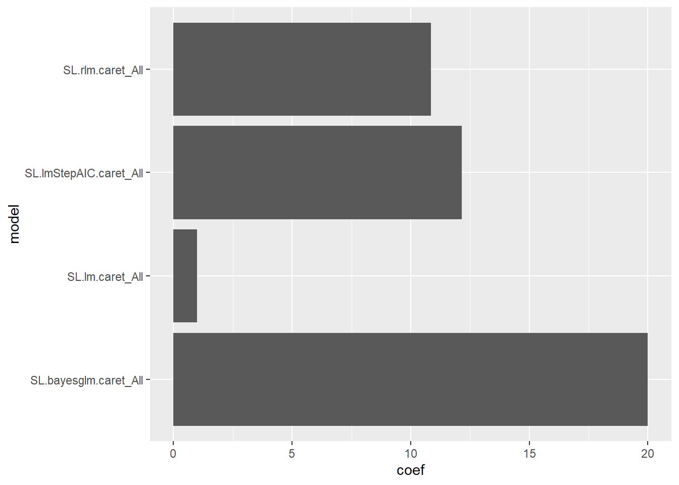
Figure 1: The sum of the per cent that the model was used by the SuperLearner
The sum of the strongest feature for every occupational group.
summary_table %>%
  arrange(desc(importance)) %>%
  group_by(ssyk) %>%
  slice(1) %>%
  ggplot (aes(importance, feature)) +
geom_col () 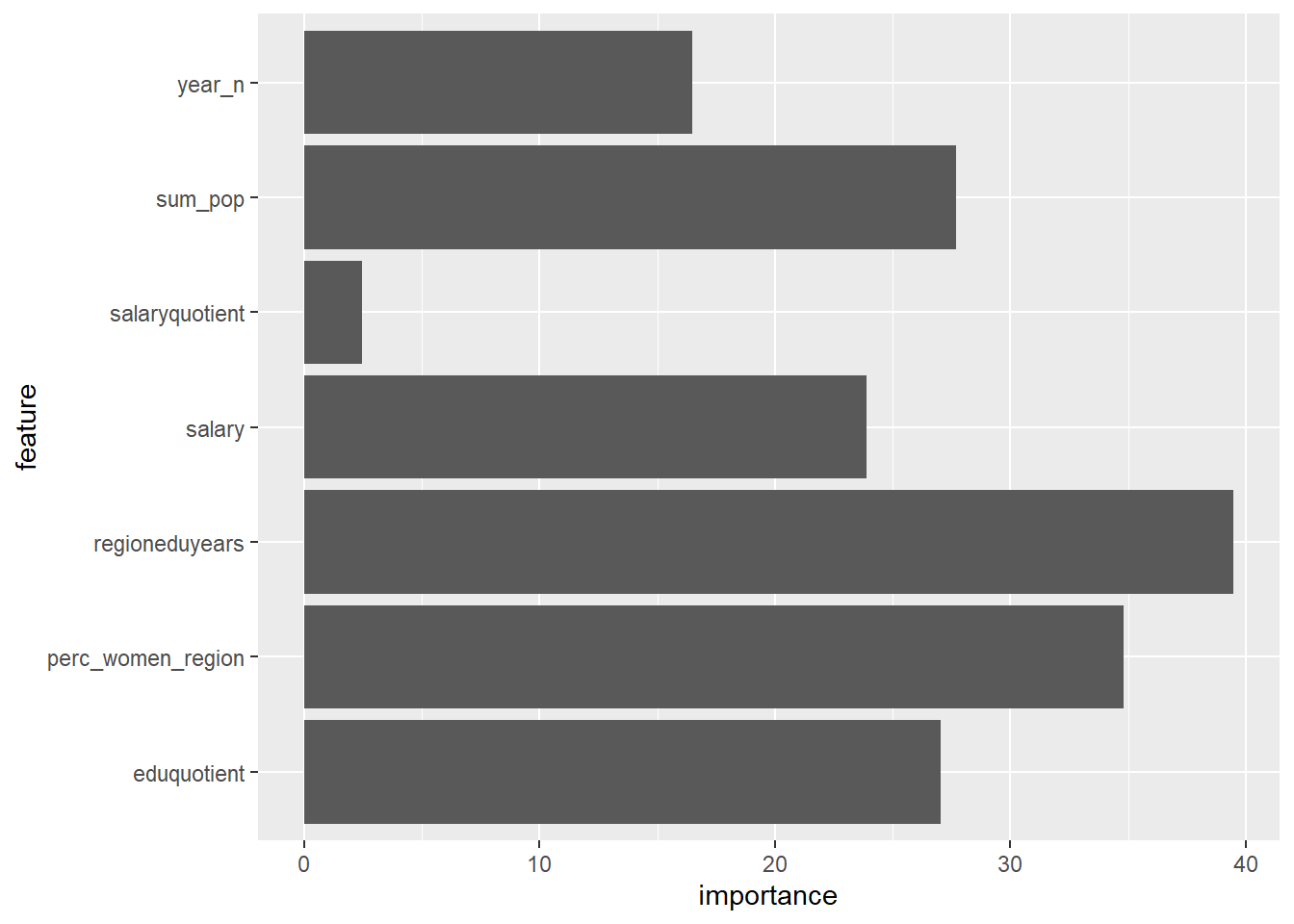
Figure 2: The sum of the strongest feature for every occupational group
Let’s see what we have found. First, check the occupation groups with a single feature that is significantly stronger than all other features. Linear models will not be suitable for all occupational groups implying that the model will not have a high R squared value.
A strong signal, the average number of education years in the region, Personal care workers in health services
temp <- filter(tb_unique, `occuptional  (SSYK 2012)` == "532 Personal care workers in health services")

model <- lm(perc_women_eng_region ~ regioneduyears, weights = suming, data = temp)

temp %>%
  ggplot () +
    geom_jitter (mapping = aes(x = regioneduyears, y = perc_women_eng_region, colour = suming)) +
    geom_abline (slope = model$coefficients[2], intercept = model$coefficients[1])  +
    labs(
      x = "Education years",
      y = "Per cent of women in the occupation"
    )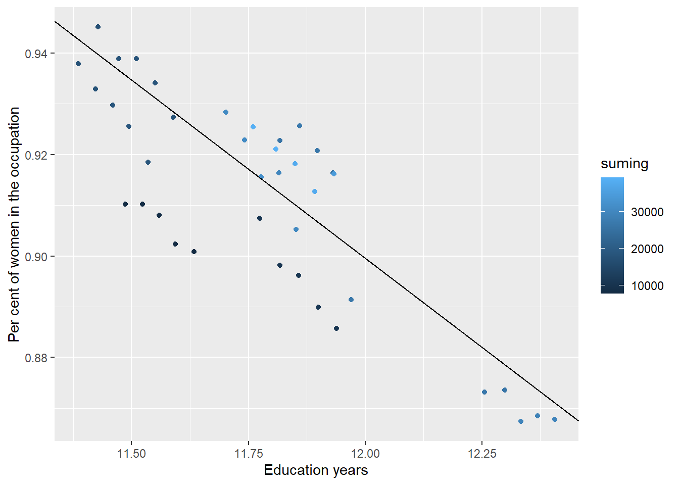
Figure 3: Personal care workers in health services, Year 2014 - 2018
summary(model)$adj.r.squared## [1] 0.7732263anova(model)## Analysis of Variance Table
##
## Response: perc_women_eng_region
## Df Sum Sq Mean Sq F value Pr(>F)
## regioneduyears 1 315.573 315.573 133.98 5.039e-14 ***
## Residuals 38 89.506 2.355
## ---
## Signif. codes: 0 '***' 0.001 '**' 0.01 '*' 0.05 '.' 0.1 ' ' 1postResample(pred = predict(model), obs = temp$perc_women_eng_region)## RMSE Rsquared MAE
## 0.01225219 0.69069055 0.01023249A strong signal, the average number of education years in the region, Medical doctors
temp <- filter(tb_unique, `occuptional  (SSYK 2012)` == "221 Medical doctors")

model <- lm(perc_women_eng_region ~ regioneduyears, weights = suming, data = temp)

temp %>%
  ggplot () +
    geom_jitter (mapping = aes(x = regioneduyears, y = perc_women_eng_region, colour = suming)) +
    geom_abline(slope = model$coefficients[2], intercept = model$coefficients[1]) +
    labs(
      x = "Education years",
      y = "Per cent of women in the occupation"
    )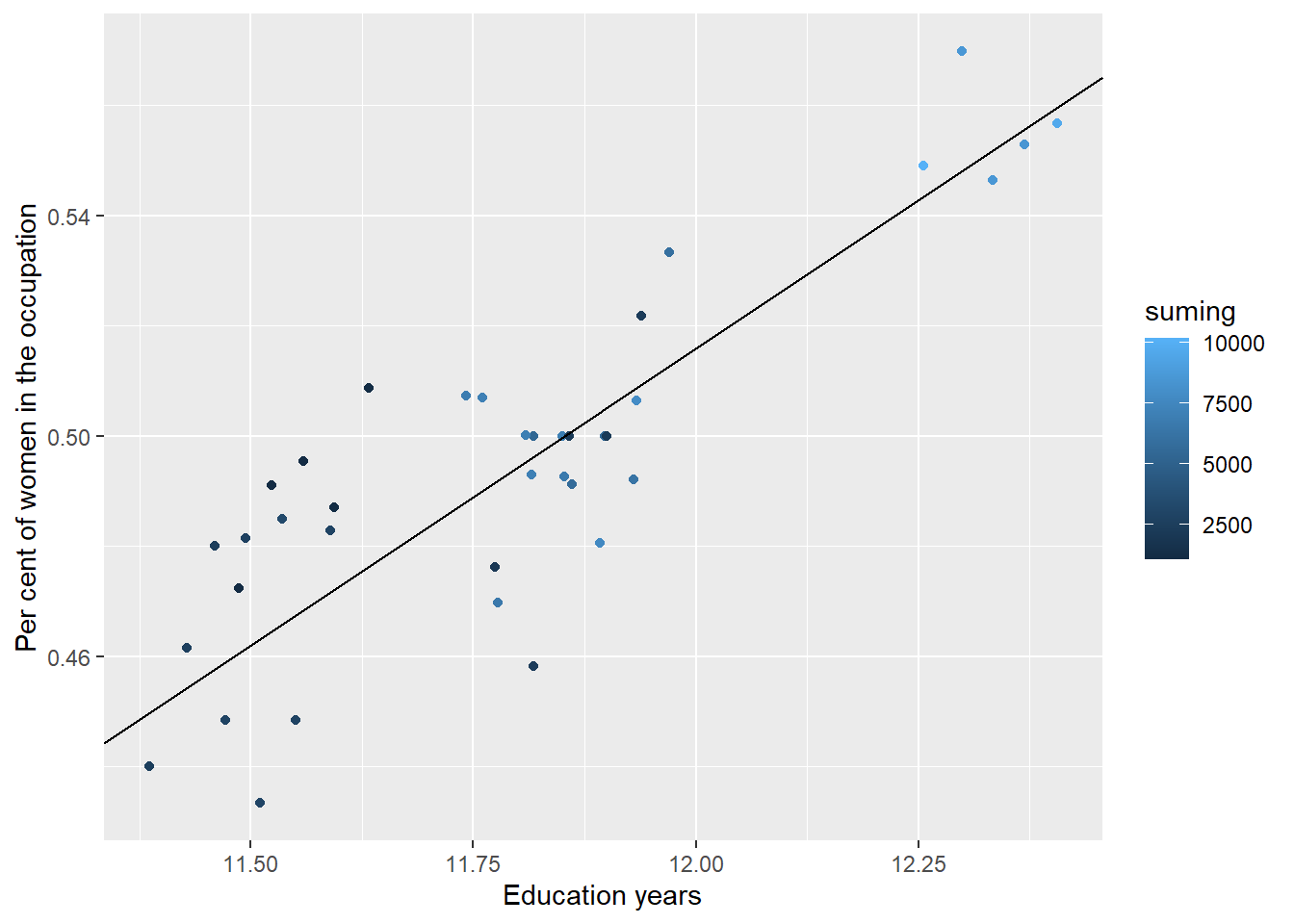
Figure 4: Medical doctors, Year 2014 - 2018
summary(model)$adj.r.squared## [1] 0.8057127anova(model)## Analysis of Variance Table
##
## Response: perc_women_eng_region
## Df Sum Sq Mean Sq F value Pr(>F)
## regioneduyears 1 164.765 164.765 154.44 1.385e-14 ***
## Residuals 36 38.407 1.067
## ---
## Signif. codes: 0 '***' 0.001 '**' 0.01 '*' 0.05 '.' 0.1 ' ' 1postResample(pred = predict(model), obs = temp$perc_women_eng_region)## RMSE Rsquared MAE
## 0.01683530 0.72088034 0.01385548A strong signal, the per cent women in the region, Insurance advisers, sales and purchasing agents
temp <- filter(tb_unique, `occuptional  (SSYK 2012)` == "332 Insurance advisers, sales and purchasing agents")

model <- lm(perc_women_eng_region ~ perc_women_region, weights = suming, data = temp)

temp %>%
  ggplot () +
    geom_jitter (mapping = aes(x = perc_women_region, y = perc_women_eng_region, colour = suming)) +
    geom_abline(slope = model$coefficients[2], intercept = model$coefficients[1]) +
    labs(
      x = "Per cent of women in the region",
      y = "Per cent of women in the occupation"
    )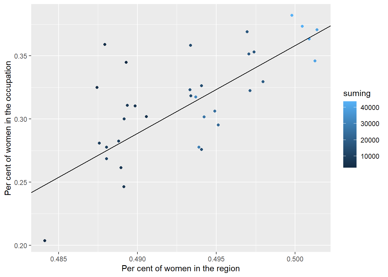
Figure 5: Insurance advisers, sales and purchasing agents, Year 2014 - 2018
summary(model)$adj.r.squared## [1] 0.6283407anova(model)## Analysis of Variance Table
##
## Response: perc_women_eng_region
## Df Sum Sq Mean Sq F value Pr(>F)
## perc_women_region 1 529.66 529.66 56.791 1.395e-08 ***
## Residuals 32 298.45 9.33
## ---
## Signif. codes: 0 '***' 0.001 '**' 0.01 '*' 0.05 '.' 0.1 ' ' 1postResample(pred = predict(model), obs = temp$perc_women_eng_region)## RMSE Rsquared MAE
## 0.02935038 0.49206133 0.02250770Two strong signals, population size in the region and the average number of education years in the region, Engineering professionals
temp <- filter(tb_unique, `occuptional  (SSYK 2012)` == "214 Engineering professionals")

s3d <- scatterplot3d(
  temp$sum_pop,
  temp$regioneduyears,
  temp$perc_women_eng_region,
  type = "h",
  color = "blue",
  xlab = "Population in region",
  ylab = "Education years",
  zlab = "Per cent of women in the occupation")

model <- lm(perc_women_eng_region ~ sum_pop + regioneduyears, weights = suming, data = temp)

s3d$plane3d(model)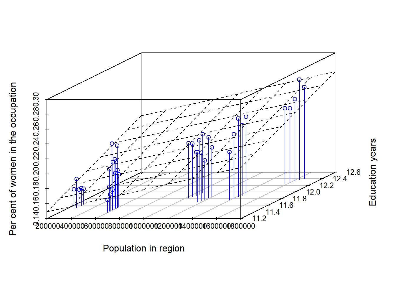
Figure 6: Engineering professionals, Year 2014 - 2018
summary(model)$adj.r.squared## [1] 0.8121964anova(model)## Analysis of Variance Table
##
## Response: perc_women_eng_region
## Df Sum Sq Mean Sq F value Pr(>F)
## sum_pop 1 255.902 255.902 144.321 5.673e-14 ***
## regioneduyears 1 31.373 31.373 17.693 0.0001712 ***
## Residuals 35 62.060 1.773
## ---
## Signif. codes: 0 '***' 0.001 '**' 0.01 '*' 0.05 '.' 0.1 ' ' 1postResample(pred = predict(model), obs = temp$perc_women_eng_region)## RMSE Rsquared MAE
## 0.012229213 0.835386966 0.009935413Two strong signals, population size in the region and the per cent women in the region, Insurance advisers, sales and purchasing agents
temp <- filter(tb_unique, `occuptional  (SSYK 2012)` == "332 Insurance advisers, sales and purchasing agents")

s3d <- scatterplot3d(
  temp$sum_pop,
  temp$perc_women_region,
  temp$perc_women_eng_region,
  type = "h",
  color = "blue",
  xlab = "Population in region",
  ylab = "Per cent of women in the region",
  zlab = "Per cent of women in the occupation")

model <- lm(perc_women_eng_region ~ sum_pop + perc_women_region, weights = suming, data = temp)

s3d$plane3d(model)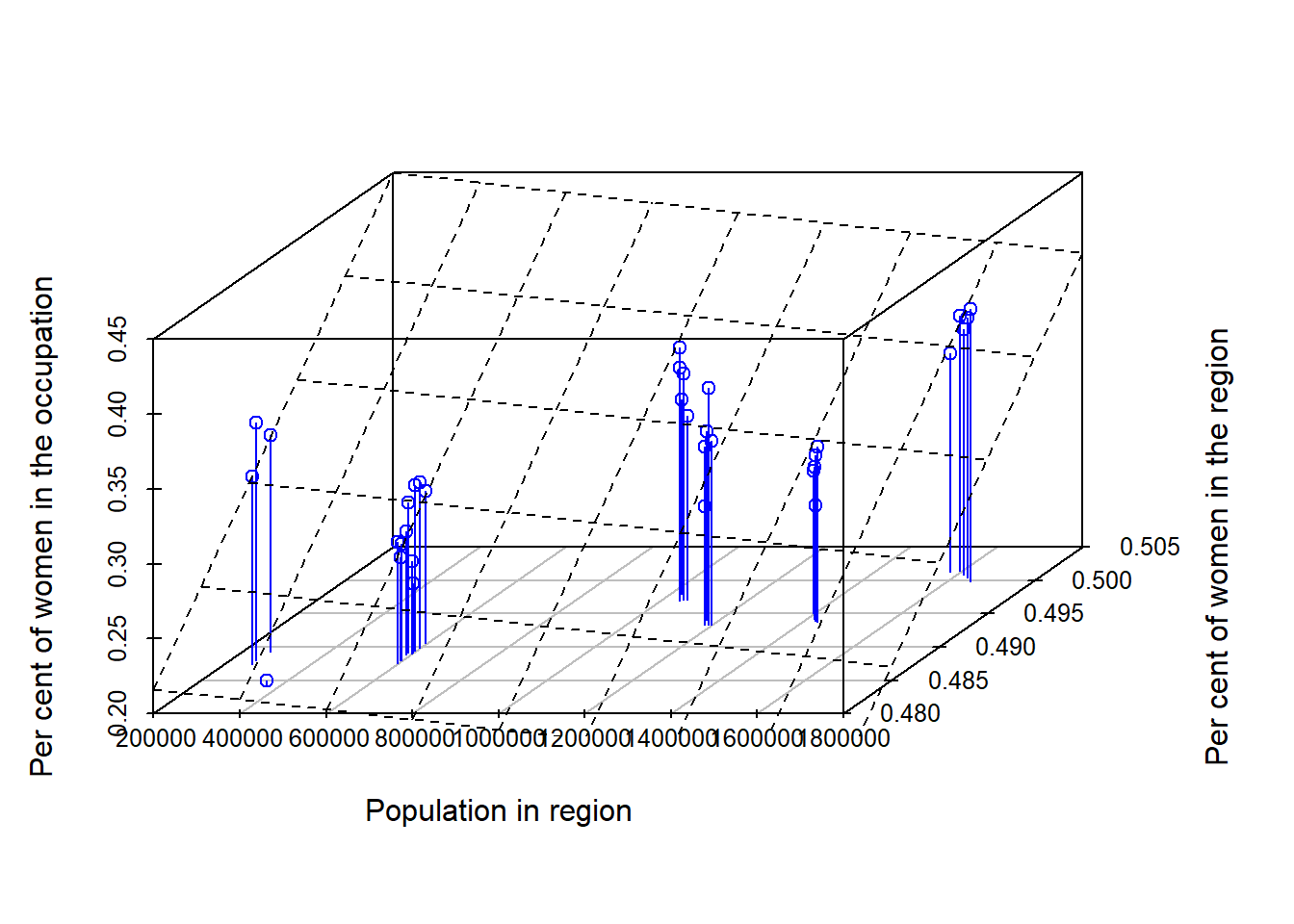
Figure 7: Insurance advisers, sales and purchasing agents, Year 2014 - 2018
summary(model)$adj.r.squared## [1] 0.6525952anova(model)## Analysis of Variance Table
##
## Response: perc_women_eng_region
## Df Sum Sq Mean Sq F value Pr(>F)
## sum_pop 1 263.40 263.403 30.214 5.168e-06 ***
## perc_women_region 1 294.45 294.455 33.776 2.099e-06 ***
## Residuals 31 270.25 8.718
## ---
## Signif. codes: 0 '***' 0.001 '**' 0.01 '*' 0.05 '.' 0.1 ' ' 1postResample(pred = predict(model), obs = temp$perc_women_eng_region)## RMSE Rsquared MAE
## 0.02638844 0.57325855 0.02034915Two strong signals, year and the per cent women in the region, Physical and engineering science technicians
temp <- filter(tb_unique, `occuptional  (SSYK 2012)` == "311 Physical and engineering science technicians")

s3d <- scatterplot3d(
  temp$year_n,
  temp$perc_women_region,
  temp$perc_women_eng_region,
  type = "h",
  color = "blue",
  xlab = "Year",
  ylab = "Per cent of women in the region",
  zlab = "Per cent of women in the occupation")

model <- lm(perc_women_eng_region ~ year_n + perc_women_region, weights = suming, data = temp)

s3d$plane3d(model)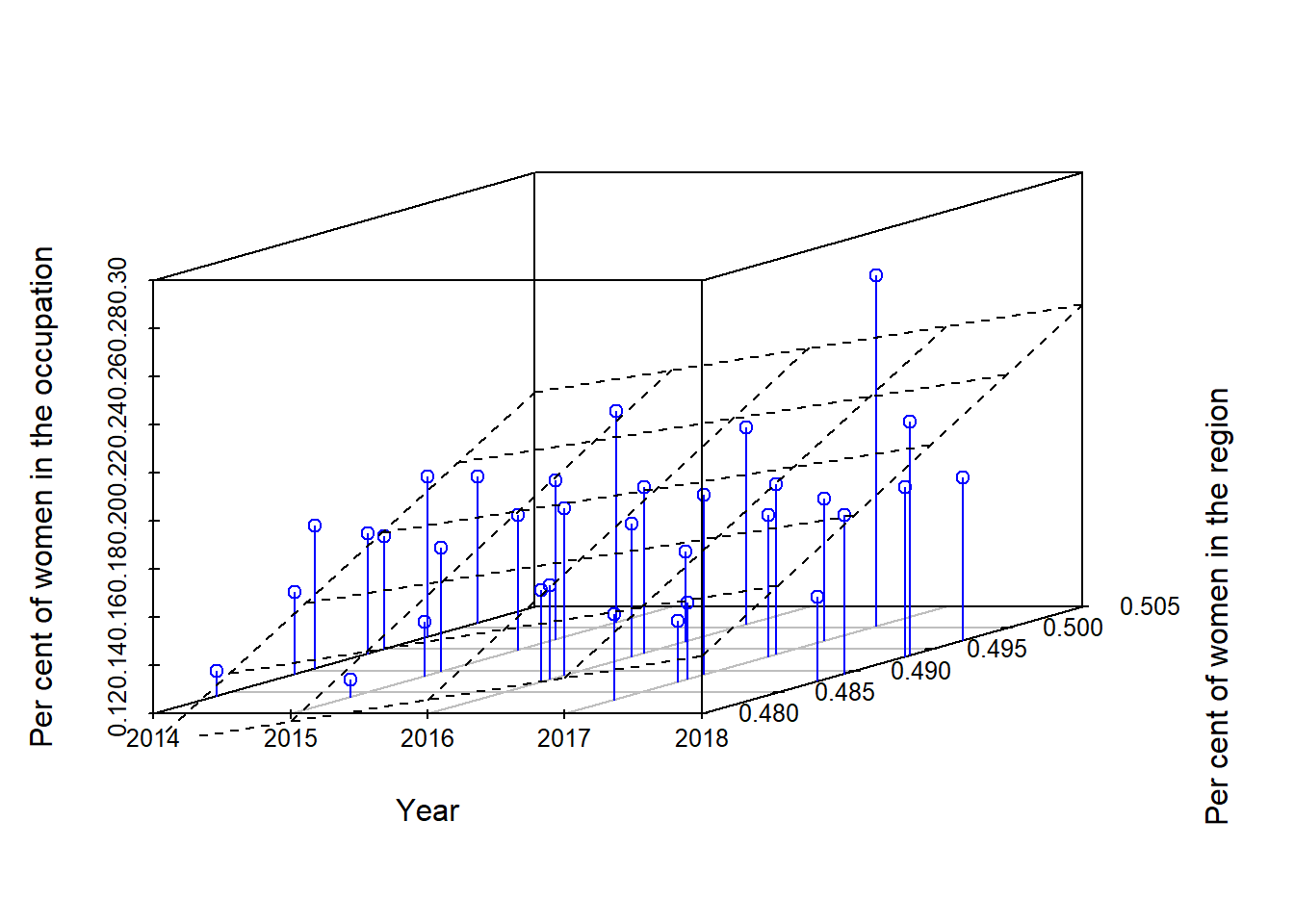
Figure 8: Physical and engineering science technicians, Year 2014 - 2018
summary(model)$adj.r.squared## [1] 0.5373011anova(model)## Analysis of Variance Table
##
## Response: perc_women_eng_region
## Df Sum Sq Mean Sq F value Pr(>F)
## year_n 1 32.63 32.630 7.6503 0.009621 **
## perc_women_region 1 134.39 134.393 31.5091 4.127e-06 ***
## Residuals 30 127.96 4.265
## ---
## Signif. codes: 0 '***' 0.001 '**' 0.01 '*' 0.05 '.' 0.1 ' ' 1postResample(pred = predict(model), obs = temp$perc_women_eng_region)## RMSE Rsquared MAE
## 0.01695193 0.59082239 0.01266243Two strong signals, year and salary, Naprapaths, physiotherapists, occupational therapists
temp <- filter(tb_unique, `occuptional  (SSYK 2012)` == "227 Naprapaths, physiotherapists, occupational therapists")

s3d <- scatterplot3d(
  temp$year_n,
  temp$salary,
  temp$perc_women_eng_region,
  type = "h",
  color = "blue",
  xlab = "Year",
  ylab = "Salary",
  zlab = "Per cent of women in the occupation")

model <- lm(perc_women_eng_region ~ year_n + salary, weights = suming, data = temp)

s3d$plane3d(model)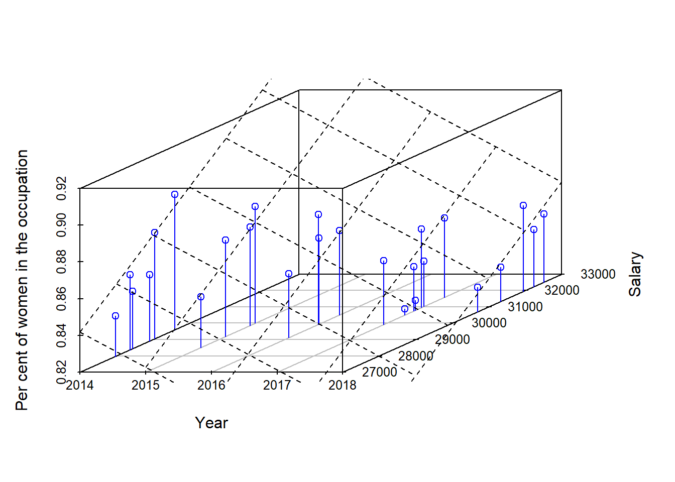
Figure 9: Naprapaths, physiotherapists, occupational therapists, Year 2014 - 2018
summary(model)$adj.r.squared## [1] 0.5269917anova(model)## Analysis of Variance Table
##
## Response: perc_women_eng_region
## Df Sum Sq Mean Sq F value Pr(>F)
## year_n 1 5.8240 5.8240 16.077 0.0005492 ***
## salary 1 4.9902 4.9902 13.776 0.0011481 **
## Residuals 23 8.3317 0.3622
## ---
## Signif. codes: 0 '***' 0.001 '**' 0.01 '*' 0.05 '.' 0.1 ' ' 1postResample(pred = predict(model), obs = temp$perc_women_eng_region)## RMSE Rsquared MAE
## 0.01261698 0.46523146 0.01003402