The publically available datasets from Statistics Sweden are aggregated tables. Groups with fewer than five records are filtered out not to have any individual data being made public.
In this post, I am going to investigate with what precision it is possible to estimate the causal effect of predictors using aggregated data. I will use the dataset CPS1988 which is contained in the AER library. Cross-section data originating from the March 1988 Current Population Survey by the US Census Bureau.
I will estimate the average treatment effect on wage for ethnicity and experience respectively. I will subclassify the predictors’ education and experience. I will balance on the observed confounders and make no attempts to handle unobserved covariates. I will not try to draw any conclusions on causal effects based on SUTVA assumptions.
First, define libraries and functions.
library (tidyverse)
## -- Attaching packages --------------------------------------- tidyverse 1.3.1 --
## v ggplot2 3.3.3     v purrr   0.3.4
## v tibble  3.1.0     v dplyr   1.0.5
## v tidyr   1.1.3     v stringr 1.4.0
## v readr   1.4.0     v forcats 0.5.1
## Warning: package 'ggplot2' was built under R version 4.0.3
## Warning: package 'tibble' was built under R version 4.0.5
## Warning: package 'tidyr' was built under R version 4.0.5
## Warning: package 'readr' was built under R version 4.0.3
## Warning: package 'dplyr' was built under R version 4.0.5
## Warning: package 'forcats' was built under R version 4.0.3
## -- Conflicts ------------------------------------------ tidyverse_conflicts() --
## x dplyr::filter() masks stats::filter()
## x dplyr::lag()    masks stats::lag()
library (AER)
## Warning: package 'AER' was built under R version 4.0.5
## Loading required package: car
## Warning: package 'car' was built under R version 4.0.3
## Loading required package: carData
## Warning: package 'carData' was built under R version 4.0.3
##
## Attaching package: 'car'
## The following object is masked from 'package:dplyr':
##
##     recode
## The following object is masked from 'package:purrr':
##
##     some
## Loading required package: lmtest
## Warning: package 'lmtest' was built under R version 4.0.4
## Loading required package: zoo
## Warning: package 'zoo' was built under R version 4.0.5
##
## Attaching package: 'zoo'
## The following objects are masked from 'package:base':
##
##     as.Date, as.Date.numeric
## Loading required package: sandwich
## Warning: package 'sandwich' was built under R version 4.0.3
## Loading required package: survival
## Warning: package 'survival' was built under R version 4.0.5
library (bnlearn)
## Warning: package 'bnlearn' was built under R version 4.0.3
library (PerformanceAnalytics)
## Loading required package: xts
## Warning: package 'xts' was built under R version 4.0.3
##
## Attaching package: 'xts'
## The following objects are masked from 'package:dplyr':
##
##     first, last
##
## Attaching package: 'PerformanceAnalytics'
## The following object is masked from 'package:graphics':
##
##     legend
library (tableone)
## Warning: package 'tableone' was built under R version 4.0.4
library (Matching)
## Warning: package 'Matching' was built under R version 4.0.5
## Loading required package: MASS
##
## Attaching package: 'MASS'
## The following object is masked from 'package:dplyr':
##
##     select
## ##
## ##  Matching (Version 4.9-9, Build Date: 2021-03-15)
## ##  See http://sekhon.berkeley.edu/matching for additional documentation.
## ##  Please cite software as:
## ##   Jasjeet S. Sekhon. 2011. ``Multivariate and Propensity Score Matching
## ##   Software with Automated Balance Optimization: The Matching package for R.''
## ##   Journal of Statistical Software, 42(7): 1-52.
## ##
library (WeightIt)
## Warning: package 'WeightIt' was built under R version 4.0.5
library (lavaan)
## Warning: package 'lavaan' was built under R version 4.0.5
## This is lavaan 0.6-8
## lavaan is FREE software! Please report any bugs.
library (tidySEM)
## Registered S3 methods overwritten by 'tidySEM':
##   method              from
##   print.mplus.model   MplusAutomation
##   print.mplusObject   MplusAutomation
##   summary.mplus.model MplusAutomation
##
## Attaching package: 'tidySEM'
## The following objects are masked from 'package:bnlearn':
##
##     nodes, nodes<-
library (cobalt)
## Warning: package 'cobalt' was built under R version 4.0.4
##  cobalt (Version 4.3.1, Build Date: 2021-03-30 09:50:18 UTC)
library (jtools)
## Warning: package 'jtools' was built under R version 4.0.5
##
## Attaching package: 'jtools'
## The following object is masked from 'package:tidySEM':
##
##     get_data

# Argument: Vector with binned values; Value: Numeric vector where each value is the mean of the binwidth
unbin_bin <- function(x){
  unbin_x <- function(x) (parse_number(unlist(strsplit(as.character(x), ",")))[1] + parse_number(unlist(strsplit(as.character(x), ",")))[2])/2

  unlist(map(x, unbin_x))
}

data(CPS1988)

CPS1988_n <- CPS1988 %>%
  mutate(education = as.numeric(education)) %>%
  mutate(experience = as.numeric(experience)) %>%
  mutate(region = as.numeric(region)) %>%
  mutate(smsa = as.numeric(smsa)) %>%
  mutate(parttime = as.numeric(parttime)) %>%
  mutate(ethnicity = as.numeric(ethnicity))
The correlation chart shows that many predictors are correlated with the response variable but also that many predictors are correlated with each other.
chart.Correlation(CPS1988_n, histogram = TRUE, pch = 19)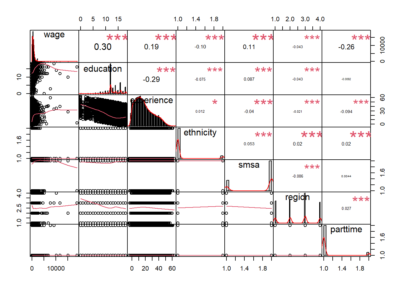
A Directed Ascyclical Graph (DAG) is a useful tool to identify backdoor paths, confounders, mediators and colliders. A DAG is usually constructed by expert knowledge in the problem domain. There are also algorithms for Bayesian networks that can estimate a DAG based on the statistical properties of the data, these estimations need to be validated against expert knowledge. I will estimate a DAG using a Bayesian network, the Hill Climbing (HC) algorithm.
hcmodel <- hc(CPS1988 %>%
  mutate(education = as.numeric(education)) %>%
  mutate(experience = as.numeric(experience)))

plot(hcmodel)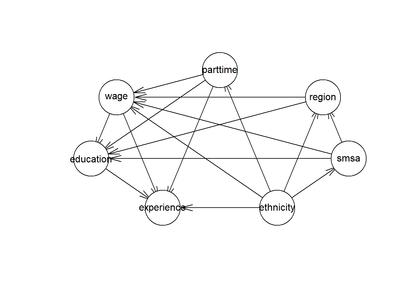
Structural Equation Modeling (SEM) is a tool to represent a system of regressions. I will use Lavaan to represent the DAG from the Bayesian network above.
semmodel = '
  education ~ wage
  wage ~ parttime
  experience ~ wage
  experience ~ parttime
  wage ~ ethnicity
  region ~ ethnicity
  region ~ smsa
  wage ~ smsa
  wage ~ region
  education ~ region
  education ~ parttime
  education ~ smsa
  smsa ~ ethnicity
  experience ~ education
  experience ~ ethnicity
  parttime ~ ethnicity
  '

semfit <- sem(semmodel,
  data =  CPS1988_n)
## Warning in lav_data_full(data = data, group = group, cluster = cluster, : lavaan
## WARNING: some observed variances are (at least) a factor 1000 times larger than
## others; use varTable(fit) to investigate

graph_sem(model = semfit)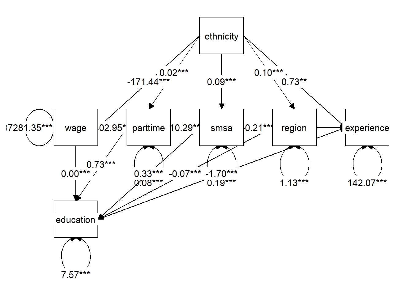
Since ethnicity is a binary variable I will use the Match algorithm to find individuals that are as similar as possible from the two groups African American and Caucasian. I will do a greedy matching based on Mahalanobis distance.
xvars <- c("education", "experience", "smsa", "region", "parttime")

print(CreateTableOne(vars = xvars, strata = "ethnicity", data = CPS1988, test = FALSE), smd = TRUE)
##                         Stratified by ethnicity
##                          cauc          afam          SMD
##   n                      25923          2232
##   education (mean (SD))  13.13 (2.90)  12.33 (2.77)   0.284
##   experience (mean (SD)) 18.15 (13.04) 18.74 (13.51)  0.044
##   smsa = yes (%)         19095 (73.7)   1837 (82.3)   0.210
##   region (%)                                          0.644
##      northeast            6073 (23.4)    368 (16.5)
##      midwest              6486 (25.0)    377 (16.9)
##      south                7468 (28.8)   1292 (57.9)
##      west                 5896 (22.7)    195 ( 8.7)
##   parttime = yes (%)      2280 ( 8.8)    244 (10.9)   0.072

greedymatch <- Match(Tr = as.integer(CPS1988$ethnicity) - 1, M = 1, X = data.frame(data.matrix(CPS1988[xvars])), replace = FALSE)

matched <- CPS1988[unlist(greedymatch[c("index.treated", "index.control")]), ]

print(CreateTableOne(vars = xvars, strata = "ethnicity", data = matched, test = FALSE), smd = TRUE)
##                         Stratified by ethnicity
##                          cauc          afam          SMD
##   n                       2232          2232
##   education (mean (SD))  12.33 (2.76)  12.33 (2.77)   0.001
##   experience (mean (SD)) 18.71 (13.44) 18.74 (13.51)  0.003
##   smsa = yes (%)          1837 (82.3)   1837 (82.3)  <0.001
##   region (%)                                          0.003
##      northeast             368 (16.5)    368 (16.5)
##      midwest               375 (16.8)    377 (16.9)
##      south                1293 (57.9)   1292 (57.9)
##      west                  196 ( 8.8)    195 ( 8.7)
##   parttime = yes (%)       244 (10.9)    244 (10.9)  <0.001

matched <- matched %>% mutate(ethnicity_n = as.integer(ethnicity) - 1)

t.test(matched$wage[matched$ethnicity_n == 1] - matched$wage[matched$ethnicity_n == 0])
##
##  One Sample t-test
##
## data:  matched$wage[matched$ethnicity_n == 1] - matched$wage[matched$ethnicity_n == 0]
## t = -12.989, df = 2231, p-value < 2.2e-16
## alternative hypothesis: true mean is not equal to 0
## 95 percent confidence interval:
##  -131.18979  -96.77381
## sample estimates:
## mean of x
## -113.9818
Another way to estimate the causal effect of ethnicity on wage is by calculating the propensity score. By regressing on the treatment, i.e. the variable that we want to calculate the effect for, we can reduce the selection bias by balancing on the covariates. Below you can see the balancing before and after using the propensity score.
W.out <- weightit(ethnicity ~ education + experience + smsa + region + parttime,
  data = CPS1988, method = "ebal")

model_lm_ethnicity <- lm(wage ~ ethnicity, data = CPS1988, weights = W.out$weights)

bal.tab(ethnicity ~ education + experience + smsa + region + parttime,
  data = CPS1988, estimand = "ATT", m.threshold = .05)
## Balance Measures
##                     Type Diff.Un      M.Threshold.Un
## education        Contin. -0.2909 Not Balanced, >0.05
## experience       Contin.  0.0435     Balanced, <0.05
## smsa_yes          Binary  0.0864 Not Balanced, >0.05
## region_northeast  Binary -0.0694 Not Balanced, >0.05
## region_midwest    Binary -0.0813 Not Balanced, >0.05
## region_south      Binary  0.2908 Not Balanced, >0.05
## region_west       Binary -0.1401 Not Balanced, >0.05
## parttime_yes      Binary  0.0214     Balanced, <0.05
##
## Balance tally for mean differences
##                     count
## Balanced, <0.05         2
## Not Balanced, >0.05     6
##
## Variable with the greatest mean difference
##   Variable Diff.Un      M.Threshold.Un
##  education -0.2909 Not Balanced, >0.05
##
## Sample sizes
##      cauc afam
## All 25923 2232

bal.tab(W.out, m.threshold = .05, disp.v.ratio = TRUE)
## Call
##  weightit(formula = ethnicity ~ education + experience + smsa +
##     region + parttime, data = CPS1988, method = "ebal")
##
## Balance Measures
##                     Type Diff.Adj     M.Threshold V.Ratio.Adj
## education        Contin.   0.0001 Balanced, <0.05      0.7731
## experience       Contin.   0.0000 Balanced, <0.05      0.9613
## smsa_yes          Binary   0.0000 Balanced, <0.05           .
## region_northeast  Binary   0.0000 Balanced, <0.05           .
## region_midwest    Binary  -0.0000 Balanced, <0.05           .
## region_south      Binary  -0.0000 Balanced, <0.05           .
## region_west       Binary  -0.0000 Balanced, <0.05           .
## parttime_yes      Binary   0.0001 Balanced, <0.05           .
##
## Balance tally for mean differences
##                     count
## Balanced, <0.05         8
## Not Balanced, >0.05     0
##
## Variable with the greatest mean difference
##   Variable Diff.Adj     M.Threshold
##  education   0.0001 Balanced, <0.05
##
## Effective sample sizes
##                cauc   afam
## Unadjusted 25923.   2232.
## Adjusted   25833.39 1233.1
Estimate the causal effect of experience on wage by calculating the propensity score.
W.out <- weightit(experience ~ ethnicity + education + smsa + region + parttime,
  data = CPS1988, method = "ebal")

model_lm_experience <- lm(wage ~ experience, data = CPS1988, weights = W.out$weights)

bal.tab(experience  ~ ethnicity + education + smsa + region + parttime,
  data = CPS1988, estimand = "ATT", m.threshold = .05)
## Balance Measures
##                     Type Corr.Un
## ethnicity_afam    Binary  0.0121
## education        Contin. -0.2867
## smsa_yes          Binary -0.0397
## region_northeast  Binary  0.0251
## region_midwest    Binary -0.0166
## region_south      Binary  0.0114
## region_west       Binary -0.0212
## parttime_yes      Binary -0.0942
##
## Sample sizes
##     Total
## All 28155

bal.tab(W.out, m.threshold = .05, disp.v.ratio = TRUE)
## Call
##  weightit(formula = experience ~ ethnicity + education + smsa +
##     region + parttime, data = CPS1988, method = "ebal")
##
## Balance Measures
##                     Type Corr.Adj Diff.Adj     M.Threshold
## ethnicity_afam    Binary       -0       -0 Balanced, <0.05
## education        Contin.       -0        0 Balanced, <0.05
## smsa_yes          Binary       -0       -0 Balanced, <0.05
## region_northeast  Binary        0        0 Balanced, <0.05
## region_midwest    Binary        0        0 Balanced, <0.05
## region_south      Binary       -0       -0 Balanced, <0.05
## region_west       Binary       -0       -0 Balanced, <0.05
## parttime_yes      Binary        0        0 Balanced, <0.05
##
## Balance tally for target mean differences
##                     count
## Balanced, <0.05         8
## Not Balanced, >0.05     0
##
## Variable with the greatest target mean difference
##   Variable Diff.Adj     M.Threshold
##  education        0 Balanced, <0.05
##
## Effective sample sizes
##               Total
## Unadjusted 28155.
## Adjusted   25793.54
Let’s now investigate how aggregating the numerical predictors in the data affects the precision when estimating the causal effect on wage. I will also filter out groups with less than 5 persons in them so that any individual can not be identified in the material. The binning and filtering reduces the original dataset by 98.9 %. By expanding the reduced dataset the original dataset can be estimated.
CPS1988_refi <- CPS1988 %>%
  mutate(education = as.numeric(education)) %>%
  mutate(experience = as.numeric(experience)) %>%
  mutate(education = cut_interval(education, 5)) %>%
  mutate(experience = cut_interval(experience, 5)) %>%
  group_by(education, experience, ethnicity, smsa, region, parttime) %>%
  mutate (wage = mean(wage)) %>%
  group_by(wage, education, experience, ethnicity, smsa, region, parttime) %>%
  tally() %>%
  mutate(experience = unbin_bin(experience)) %>%
  mutate(education = unbin_bin(education)) %>%
  filter(n > 4)

dim(CPS1988_refi)
## [1] 302   8

CPS1988_refiexp <- CPS1988_refi[rep(seq(nrow(CPS1988_refi)), CPS1988_refi$n),]

dim(CPS1988_refiexp)
## [1] 27797     8
How has the reduction affected the DAG? It is not possible to use weights in the hc algorithm. Therefore I will use the expanded table based on the data in the aggregated table.
hcmodel_refiexp <- hc(dplyr::select(CPS1988_refiexp %>%
  mutate(education = as.numeric(education)) %>%
  mutate(experience = as.numeric(experience)), -n))

plot(hcmodel_refiexp)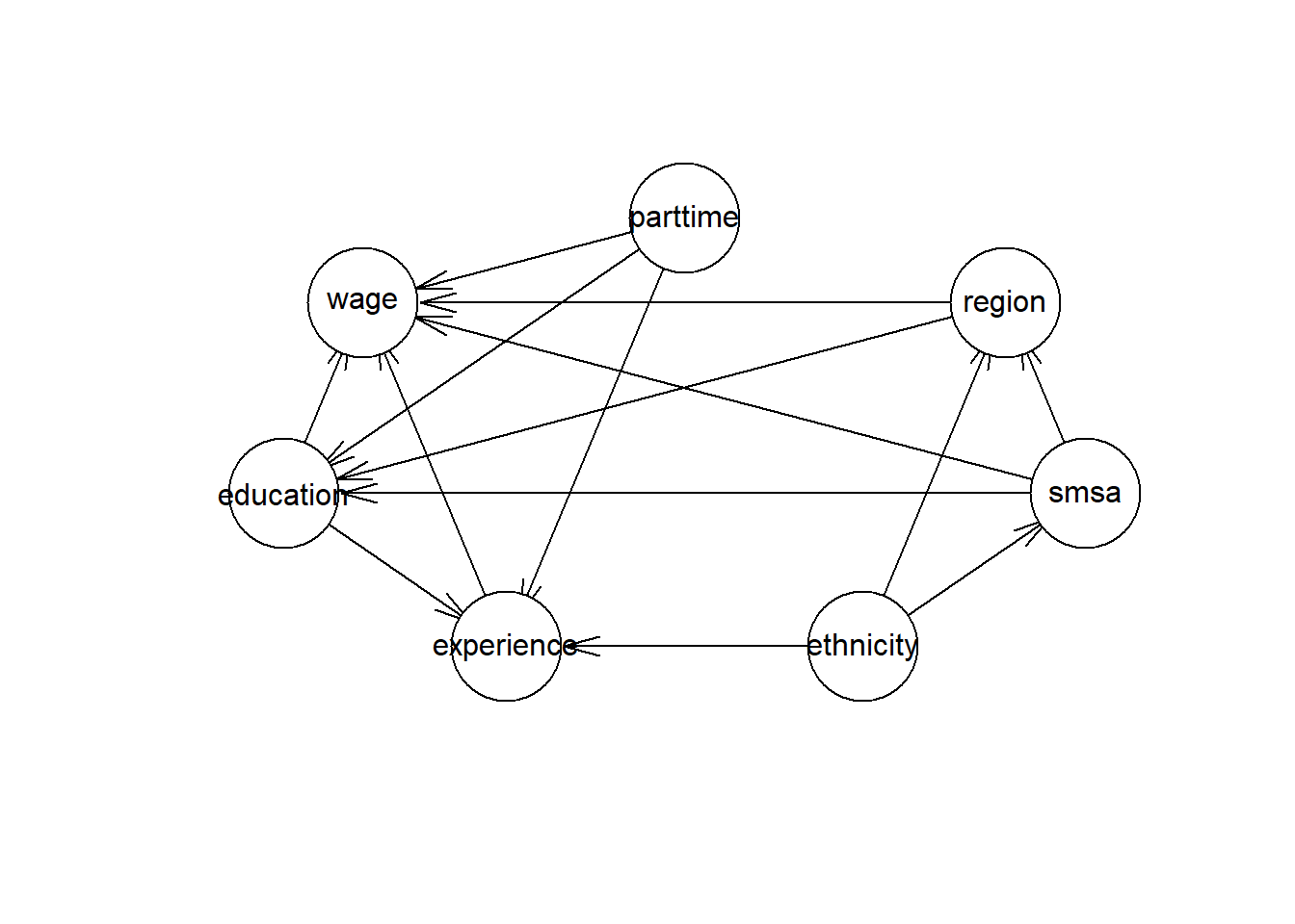
For comparison, I will plot the coefficients for ethnicity for the linear model based on the original data, aggregated data and the expanded data. I will use robust (Heteroskedasticity-Consistent) error estimates.
model <- lm(wage ~ ethnicity, data = CPS1988)

model_refi <- lm(wage ~ ethnicity, data = CPS1988_refi, weights = n)

model_refiexp <- lm(wage ~ ethnicity, data = CPS1988_refiexp)

plot_summs(model, model_refi, model_refiexp, robust = "HC1",
  model.names = c(
    "Original dataset",
    "Reduced dataset using weights",
    "Expanded dataset"))
## Loading required namespace: broom.mixed
## Warning in checkMatrixPackageVersion(): Package version inconsistency detected.
## TMB was built with Matrix version 1.3.2
## Current Matrix version is 1.2.18
## Please re-install 'TMB' from source using install.packages('TMB', type = 'source') or ask CRAN for a binary version of 'TMB' matching CRAN's 'Matrix' package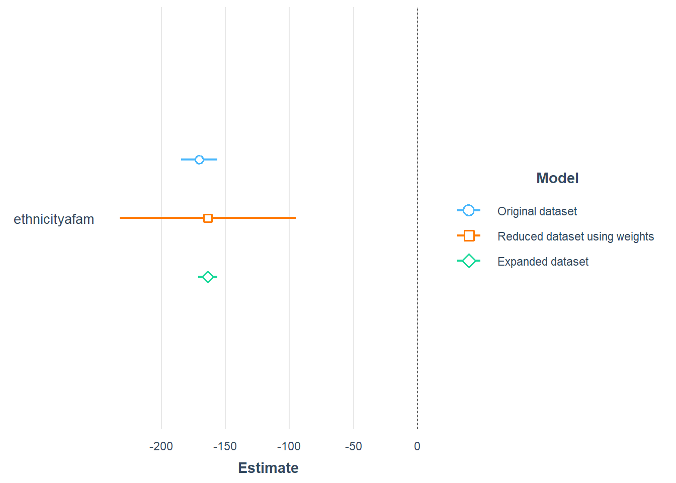
Now let’s estimate the causal effect of ethnicity on wage using propensity scores. I will use the expanded dataset since I did not get any reasonable results using the argument s.weights in weightit.
W.out <- weightit(ethnicity ~ education + experience + smsa + region + parttime,
  data = CPS1988_refiexp, method = "ebal")

model_refiexp <- lm(wage ~ ethnicity, data = CPS1988_refiexp, weights = W.out$weights)

coeftest(model_refiexp, vcov = vcovHC, type = "HC1")
##
## t test of coefficients:
##
##                Estimate Std. Error t value  Pr(>|t|)
## (Intercept)    616.8706     1.4634 421.541 < 2.2e-16 ***
## ethnicityafam -133.7648     6.1773 -21.654 < 2.2e-16 ***
## ---
## Signif. codes:  0 '***' 0.001 '**' 0.01 '*' 0.05 '.' 0.1 ' ' 1

bal.tab(ethnicity ~ education + experience + smsa + region + parttime,
  data = CPS1988_refiexp, estimand = "ATT", m.threshold = .05)
## Balance Measures
##                     Type Diff.Un      M.Threshold.Un
## education        Contin. -0.2050 Not Balanced, >0.05
## experience       Contin. -0.0567 Not Balanced, >0.05
## smsa_yes          Binary  0.0995 Not Balanced, >0.05
## region_northeast  Binary -0.0784 Not Balanced, >0.05
## region_midwest    Binary -0.0800 Not Balanced, >0.05
## region_south      Binary  0.3059 Not Balanced, >0.05
## region_west       Binary -0.1475 Not Balanced, >0.05
## parttime_yes      Binary -0.0052     Balanced, <0.05
##
## Balance tally for mean differences
##                     count
## Balanced, <0.05         1
## Not Balanced, >0.05     7
##
## Variable with the greatest mean difference
##      Variable Diff.Un      M.Threshold.Un
##  region_south  0.3059 Not Balanced, >0.05
##
## Sample sizes
##      cauc afam
## All 25732 2065

bal.tab(W.out, m.threshold = .05, disp.v.ratio = TRUE)
## Call
##  weightit(formula = ethnicity ~ education + experience + smsa +
##     region + parttime, data = CPS1988_refiexp, method = "ebal")
##
## Balance Measures
##                     Type Diff.Adj     M.Threshold V.Ratio.Adj
## education        Contin.   0.0001 Balanced, <0.05      0.6710
## experience       Contin.   0.0000 Balanced, <0.05      0.8969
## smsa_yes          Binary   0.0000 Balanced, <0.05           .
## region_northeast  Binary   0.0000 Balanced, <0.05           .
## region_midwest    Binary   0.0001 Balanced, <0.05           .
## region_south      Binary  -0.0000 Balanced, <0.05           .
## region_west       Binary  -0.0001 Balanced, <0.05           .
## parttime_yes      Binary  -0.0000 Balanced, <0.05           .
##
## Balance tally for mean differences
##                     count
## Balanced, <0.05         8
## Not Balanced, >0.05     0
##
## Variable with the greatest mean difference
##        Variable Diff.Adj     M.Threshold
##  region_midwest   0.0001 Balanced, <0.05
##
## Effective sample sizes
##               cauc    afam
## Unadjusted 25732.  2065.
## Adjusted   25650.5 1094.35

plot_summs(model_lm_ethnicity, model_refiexp, scale = TRUE, robust = "HC1",
  model.names = c(
    "Original dataset",
    "Expanded dataset"))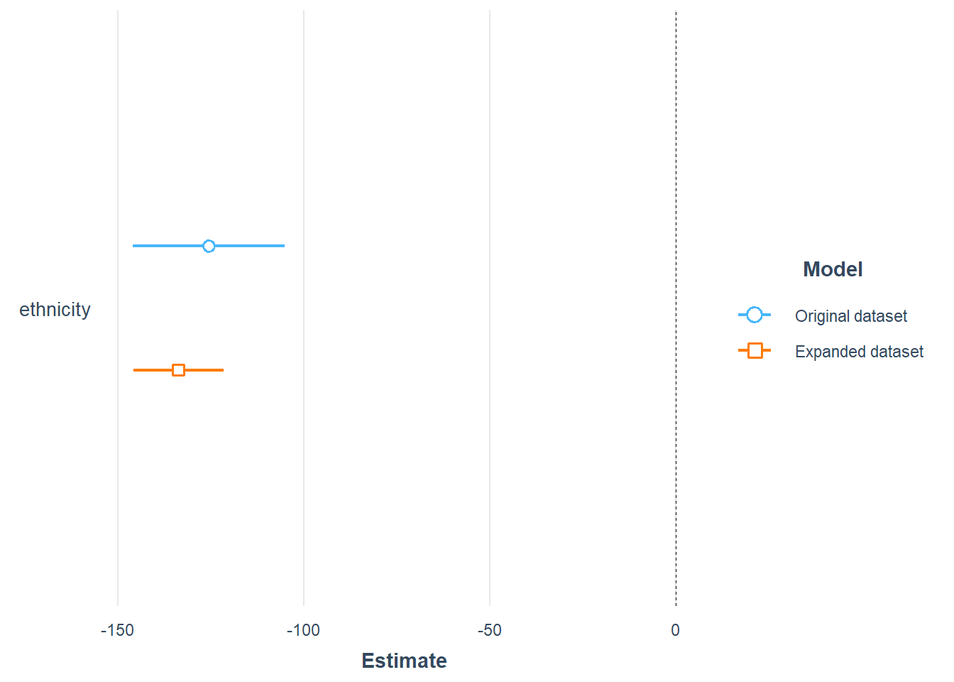
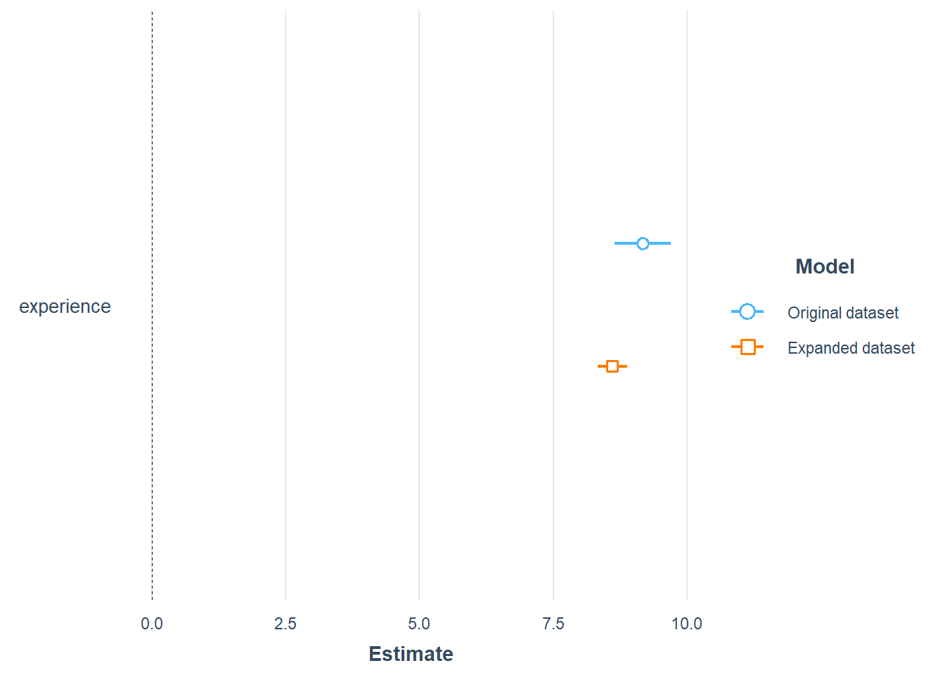
Let’s compare the coefficients for experience for the linear model based on the original data, aggregated data and the expanded data.
model <- lm(wage ~ experience, data = CPS1988)

model_refi <- lm(wage ~ experience, data = CPS1988_refi, weights = n)

model_refiexp <- lm(wage ~ experience, data = CPS1988_refiexp)

plot_summs(model, model_refi, model_refiexp, robust = "HC1",
  model.names = c(
    "Original dataset",
    "Reduced dataset using weights",
    "Expanded dataset"))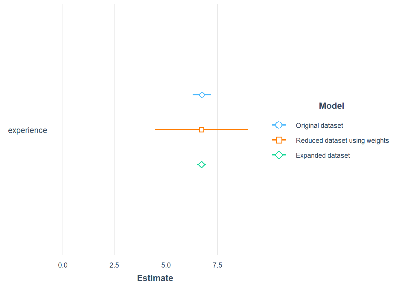
Let’s estimate the causal effect of ethnicity on wage using propensity scores. I will use the expanded dataset since I did not get any reasonable results using the argument s.wights in weightit.
W.out <- weightit(experience ~ ethnicity + education + smsa + region + parttime,
  data = CPS1988_refiexp, method = "ebal")

model_refiexp <- lm(wage ~ experience, data = CPS1988_refiexp, weights = W.out$weights)

coeftest(model_refiexp, vcov = vcovHC, type = "HC1")
##
## t test of coefficients:
##
##              Estimate Std. Error t value  Pr(>|t|)
## (Intercept) 452.45062    2.25958 200.237 < 2.2e-16 ***
## experience    8.60394    0.14098  61.029 < 2.2e-16 ***
## ---
## Signif. codes:  0 '***' 0.001 '**' 0.01 '*' 0.05 '.' 0.1 ' ' 1

bal.tab(experience ~ ethnicity + education + smsa + region + parttime,
  data = CPS1988_refiexp, estimand = "ATT", m.threshold = .05)
## Balance Measures
##                     Type Corr.Un
## ethnicity_afam    Binary -0.0143
## education        Contin. -0.2736
## smsa_yes          Binary -0.0339
## region_northeast  Binary  0.0256
## region_midwest    Binary -0.0156
## region_south      Binary  0.0092
## region_west       Binary -0.0202
## parttime_yes      Binary -0.1072
##
## Sample sizes
##     Total
## All 27797

bal.tab(W.out, m.threshold = .05, disp.v.ratio = TRUE)
## Call
##  weightit(formula = experience ~ ethnicity + education + smsa +
##     region + parttime, data = CPS1988_refiexp, method = "ebal")
##
## Balance Measures
##                     Type Corr.Adj Diff.Adj     M.Threshold
## ethnicity_afam    Binary       -0       -0 Balanced, <0.05
## education        Contin.       -0       -0 Balanced, <0.05
## smsa_yes          Binary       -0       -0 Balanced, <0.05
## region_northeast  Binary        0        0 Balanced, <0.05
## region_midwest    Binary        0        0 Balanced, <0.05
## region_south      Binary       -0       -0 Balanced, <0.05
## region_west       Binary       -0       -0 Balanced, <0.05
## parttime_yes      Binary        0       -0 Balanced, <0.05
##
## Balance tally for target mean differences
##                     count
## Balanced, <0.05         8
## Not Balanced, >0.05     0
##
## Variable with the greatest target mean difference
##   Variable Diff.Adj     M.Threshold
##  education       -0 Balanced, <0.05
##
## Effective sample sizes
##               Total
## Unadjusted 27797.
## Adjusted   25618.89

plot_summs(model_lm_experience, model_refiexp, robust = "HC1",
  model.names = c(
    "Original dataset",
"Expanded dataset")) 