In this post, I will examine Dynamic Linear Models and Time-Series Regression. I will return to data for Engineers from Statistics Sweden. Since the salaries for each year, each stratum (age group) is strongly correlated with the salary for the previous year it does not seem too distant to use a time series to represent the change of salaries throughout the period.
I will let the age represent the season in the time series. This violates the properties of a regular time series and has to be considered for the rest of the analysis. First, let´s decompose the series into its trend and seasonal patterns.
First, define libraries and functions.
library (tidyverse)
## -- Attaching packages --------------------------------------- tidyverse 1.3.1 --
## v ggplot2 3.3.3     v purrr   0.3.4
## v tibble  3.1.0     v dplyr   1.0.5
## v tidyr   1.1.3     v stringr 1.4.0
## v readr   1.4.0     v forcats 0.5.1
## Warning: package 'ggplot2' was built under R version 4.0.3
## Warning: package 'tibble' was built under R version 4.0.5
## Warning: package 'tidyr' was built under R version 4.0.5
## Warning: package 'readr' was built under R version 4.0.3
## Warning: package 'dplyr' was built under R version 4.0.5
## Warning: package 'forcats' was built under R version 4.0.3
## -- Conflicts ------------------------------------------ tidyverse_conflicts() --
## x dplyr::filter() masks stats::filter()
## x dplyr::lag()    masks stats::lag()
library(imputeTS)
## Warning: package 'imputeTS' was built under R version 4.0.5
## Registered S3 method overwritten by 'quantmod':
##   method            from
##   as.zoo.data.frame zoo
library(TSstudio)
## Warning: package 'TSstudio' was built under R version 4.0.5
library(forecast)
## Warning: package 'forecast' was built under R version 4.0.5
library(dynlm)
## Warning: package 'dynlm' was built under R version 4.0.5
## Loading required package: zoo
## Warning: package 'zoo' was built under R version 4.0.5
##
## Attaching package: 'zoo'
## The following object is masked from 'package:imputeTS':
##
##     na.locf
## The following objects are masked from 'package:base':
##
##     as.Date, as.Date.numeric
library(lmtest)
## Warning: package 'lmtest' was built under R version 4.0.4
library(sandwich)
## Warning: package 'sandwich' was built under R version 4.0.3
library(ggeffects)
## Warning: package 'ggeffects' was built under R version 4.0.5

readfile <- function (file1){
  read_csv (file1, col_types = cols(), locale = readr::locale (encoding = "latin1"), na = c("..", "NA")) %>%
    gather (starts_with("19"), starts_with("20"), key = "year", value = salary) %>%
    mutate (year_n = parse_number (year))
}

# Thanks to Grant, Stack Overflow
predNeweyWest <- function (model){
  pred_df <- data.frame(fit = predict(model))

  X_mat <- model.matrix(model)

  v_hac <- NeweyWest(model, prewhite = FALSE, adjust = TRUE)

  var_fit_hac <- rowSums((X_mat %*% v_hac) * X_mat)
  se_fit_hac <- sqrt(var_fit_hac)

  pred_df <-
    pred_df %>%
    mutate(se_fit_hac = se_fit_hac) %>%
    mutate(
      lwr_hac = fit - qt(0.975, df = model$df.residual) * se_fit_hac,
      upr_hac = fit + qt(0.975, df = model$df.residual) * se_fit_hac
    )
}

plotmodel <- function(data, pred_df, no_n = FALSE){
  if(no_n){
  bind_cols(
    data,
    pred_df
    ) %>%
      ggplot(aes(x = year_dec, y = salary, ymin = lwr_hac, ymax = upr_hac)) +
      geom_point() +
      geom_ribbon(fill = "#E41A1C", alpha = 0.3, col = NA) +
      labs(
        x = "Year",
        y = "Salary (SEK/month)",
        caption = 'Shaded region indicates HAC 95% CI.'
    )
  }
  else{
  bind_cols(
    data,
    pred_df
    ) %>%
      ggplot(aes(x = year_dec, y = salary, color = n, ymin = lwr_hac, ymax = upr_hac)) +
      geom_point() +
      geom_ribbon(fill = "#E41A1C", alpha = 0.3, col = NA) +
      labs(
        x = "Year",
        y = "Salary (SEK/month)",
        caption = 'Shaded region indicates HAC 95% CI.'
    )
  }
}

assess_model <- function(model, timeseries, data, no_n = FALSE, doexp = FALSE){
  print(summary (model))

  print(coeftest(model, vcov = NeweyWest, prewhite = F, adjust = T))

  print(checkresiduals(model))

  if(doexp){
    pred_df <- exp(predNeweyWest(model))
  } else {
    pred_df <- predNeweyWest(model)
  }

  pred_df$year_dec <- timeseries

  plotmodel(data, pred_df, no_n)
}
The data table is downloaded from Statistics Sweden. It is saved as a comma-delimited file without heading, 000000D2_20210506-201343.csv, http://www.statistikdatabasen.scb.se/pxweb/en/ssd/.
The table: Average monthly pay (total pay), non-manual workers all sectors (SLP), SEK by occupational group (SSYK), age, sex and year. SSYK 2012 214, Year 2014 - 2019
The average age within each age group is used as a numeric value for graphical presentation and the linear model.
The number of Engineers in each stratum is downloaded separately in the file 000000CZ_20210506-201420.csv.
tb <- readfile("000000D2_20210506-201343.csv") %>%
rowwise() %>%
mutate(age_l = unlist(lapply(strsplit(substr(age, 1, 5), "-"), strtoi))[1]) %>%
rowwise() %>%
mutate(age_h = unlist(lapply(strsplit(substr(age, 1, 5), "-"), strtoi))[2]) %>%
mutate(age_n = (age_l + age_h) / 2)
tbcount <- readfile("000000CZ_20210506-201420.csv")
tbcount$salary <- replace(tbcount$salary, is.na(tbcount$salary), 0)
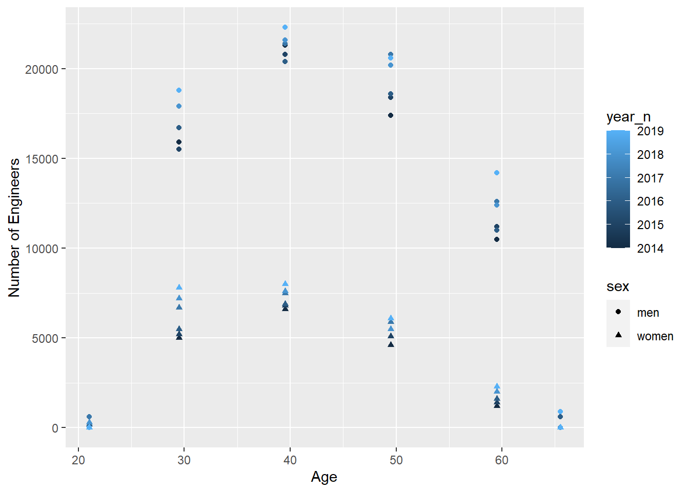
tb$n <- tbcount$salaryLet’s have a look at the age distribution for the different years for men and women.
tb %>%
  ggplot () +
    geom_point (mapping = aes(x = age_n,y = n, colour = year_n, shape = sex)) +
  labs(
    x = "Age",
    y = "Number of Engineers"
  )
Create a time series for each gender. Time series can not have missing values, Impute missing values in time series with arima model. Women don’t have any data for the age group 65-66 year, that group is filtered away.
tb_men <- filter(tb, sex == "men")

tb_women <- filter(tb, sex == "women") %>% filter(age_n != 65.5)

summary(tb_men$salary)
##    Min. 1st Qu.  Median    Mean 3rd Qu.    Max.    NA's
##   27300   36550   47100   43340   49500   52800       1

summary(tb_women$salary)
##    Min. 1st Qu.  Median    Mean 3rd Qu.    Max.    NA's
##   26600   35000   44700   41293   45900   52100       1

tbts_men <- ts(tb_men$salary, start = 2014, freq = 6) %>% na_kalman("auto.arima")

tbts_women <- ts(tb_women$salary, start = 2014, freq = 5) %>% na_kalman("auto.arima")

tb_men$salary <- as.numeric(tbts_men)

tb_women$salary <- as.numeric(tbts_women)
Let’s use the decompose function from the stats package to view the trend, seasonal and random component of the time series.
decompose(tbts_men) %>% plot()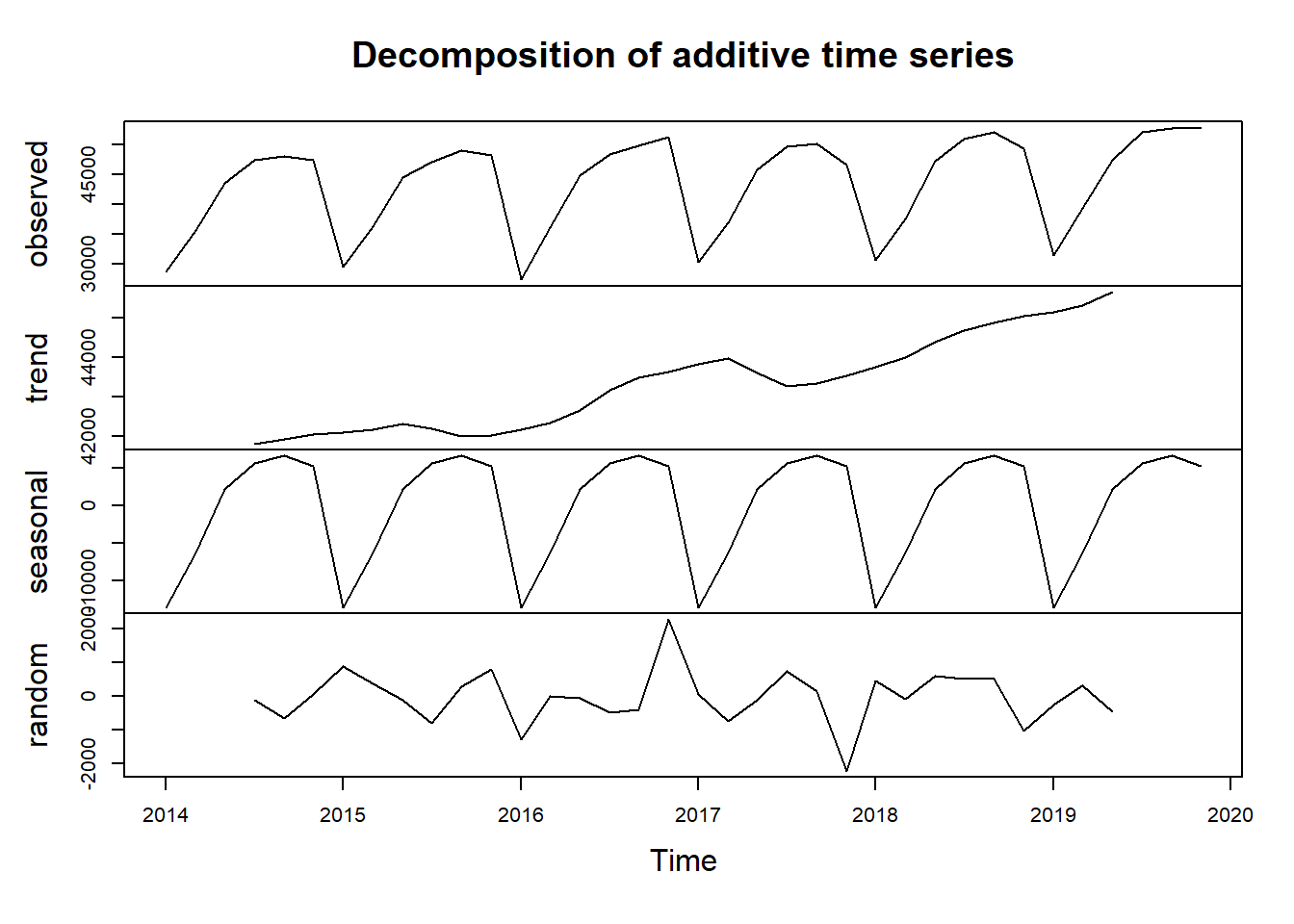
decompose(tbts_women) %>% plot()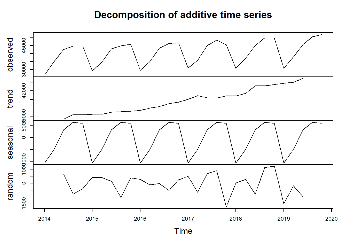
Let´s have a look at the autocorrelation for the series. As expected the series for men shows a strong correlation with its sixth lag, i.e. the same age category the year before. The series for women shows a strong correlation with its fifth lag.
acf(tbts_men, 36)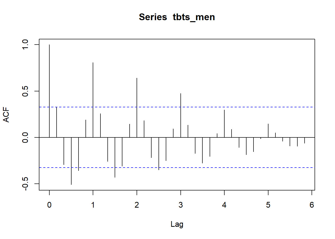
acf(tbts_women, 30)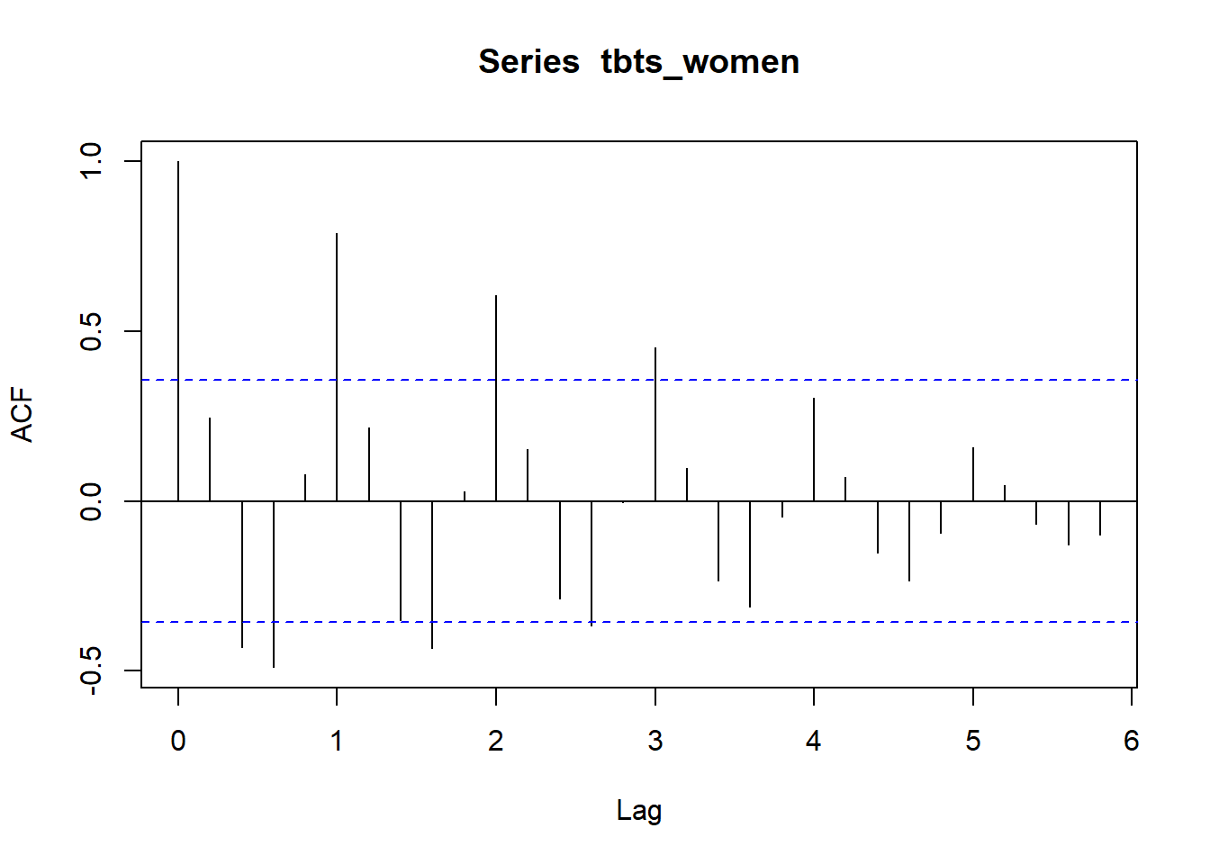
The partial autocorrelation function gives the partial correlation of a stationary time series with its own lagged values, regressed the values of the time series at all shorter lags.
pacf(tbts_men, 36)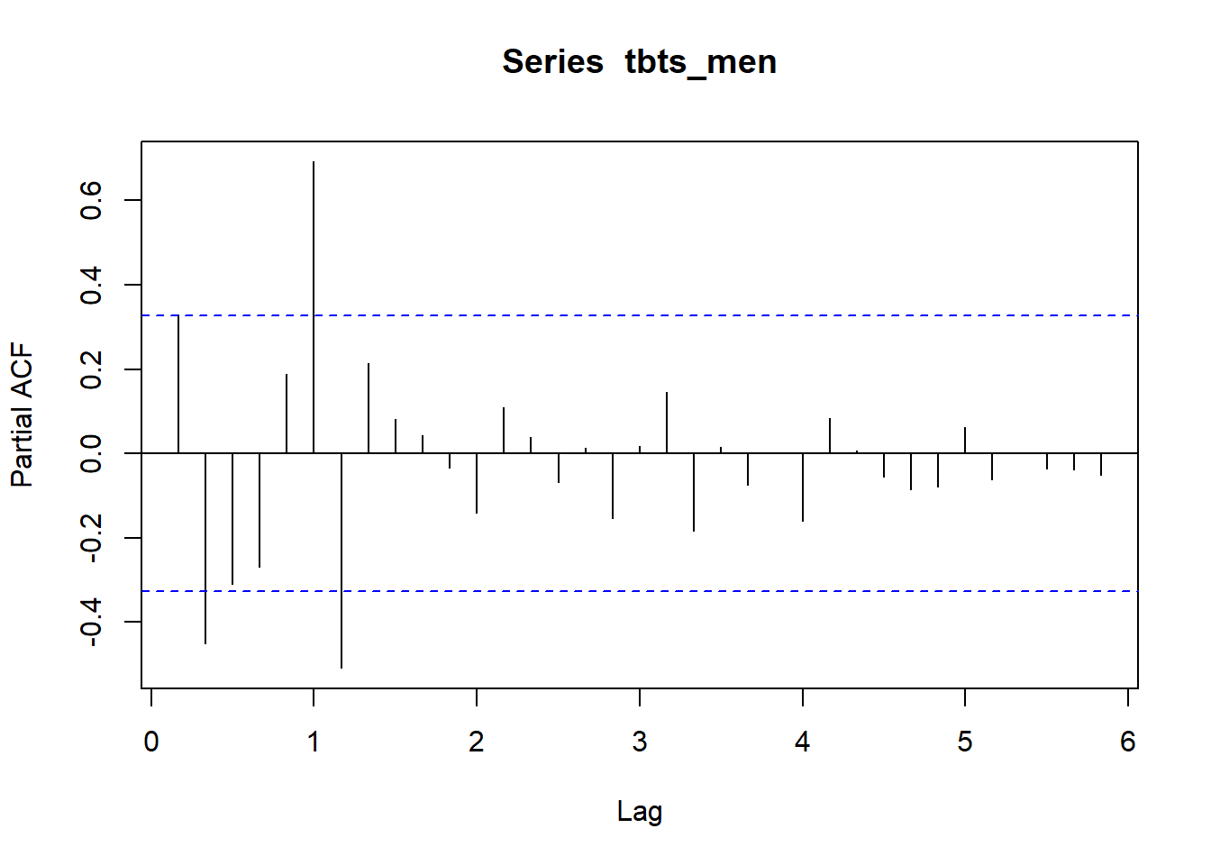
pacf(tbts_women, 36)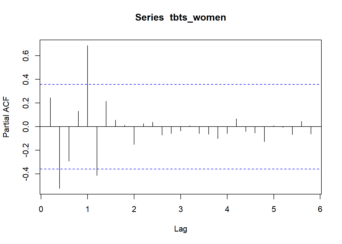
The following plot shows the correlation between the salary and its yearly lag for three years.
ts_lags(tbts_men, c(6, 12, 18))Now, let’s fit an arima model to the time series with the auto.arima from the forecast library. The summary shows that the auto.arima has identified a SAR(2) process with drift and additionally an element of random walk. The checkresiduals function plots the residuals from the arima model, the autocorrelation of the residuals and a histogram of the residual distribution. The Ljung-Box test suggests that only white noise remains in the residual. The ggseasonplot plots the salary distribution on age for the years 2014-2019, remember that we used age as a season in this approach.
arimamodel_men <- auto.arima(tbts_men)

summary(arimamodel_men)
## Series: tbts_men
## ARIMA(0,0,0)(2,1,0)[6] with drift
##
## Coefficients:
##         sar1     sar2     drift
##       -0.761  -0.6098  128.8569
## s.e.   0.158   0.1435   16.1691
##
## sigma^2 estimated as 1163963:  log likelihood=-254.04
## AIC=516.08   AICc=517.68   BIC=521.69
##
## Training set error measures:
##                     ME     RMSE      MAE        MPE    MAPE     MASE      ACF1
## Training set -25.68999 934.3299 573.1137 -0.1985635 1.37638 0.434177 0.2314468

checkresiduals(arimamodel_men)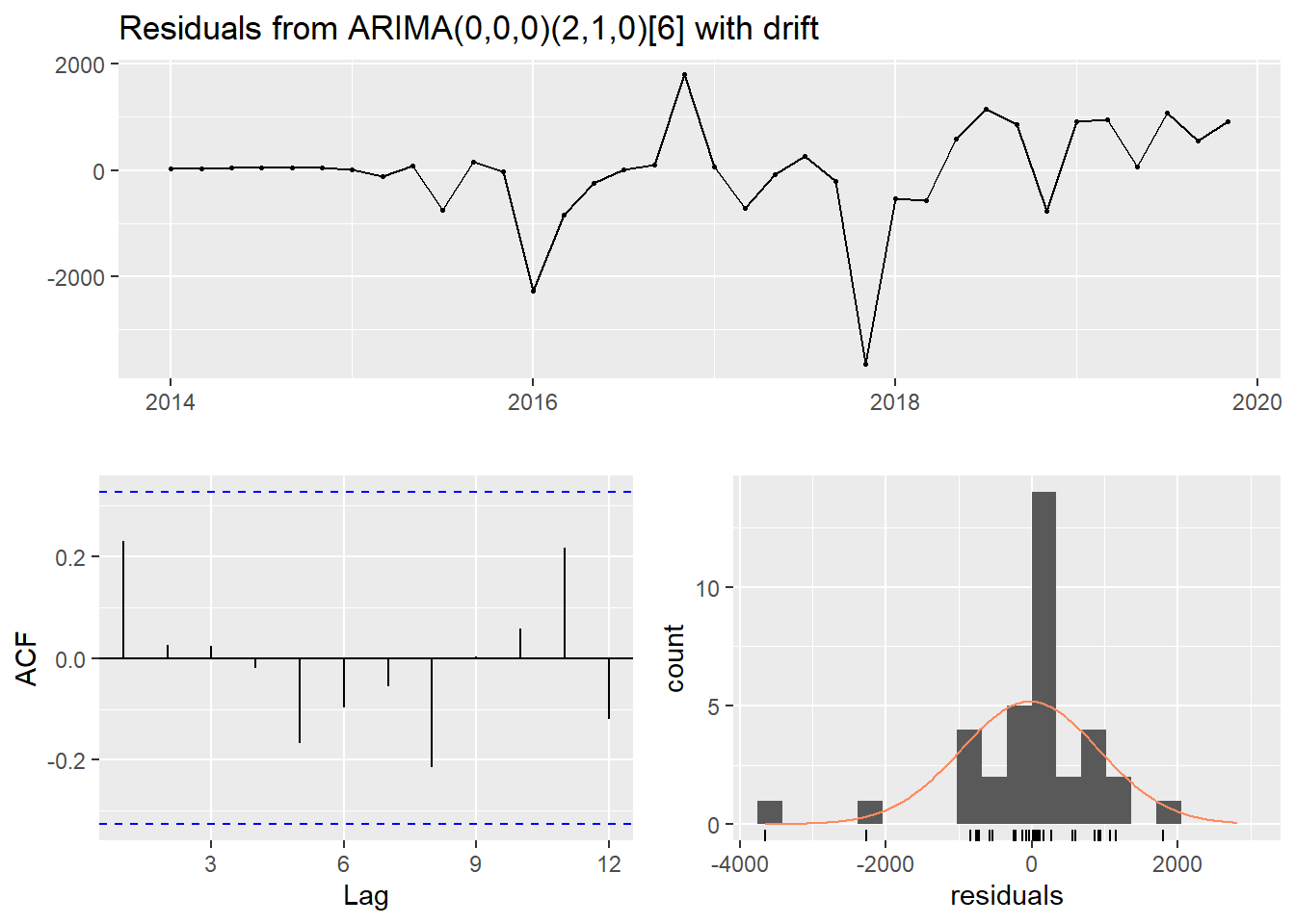
##
##  Ljung-Box test
##
## data:  Residuals from ARIMA(0,0,0)(2,1,0)[6] with drift
## Q* = 3.9755, df = 4, p-value = 0.4093
##
## Model df: 3.   Total lags used: 7

ggseasonplot(tbts_men)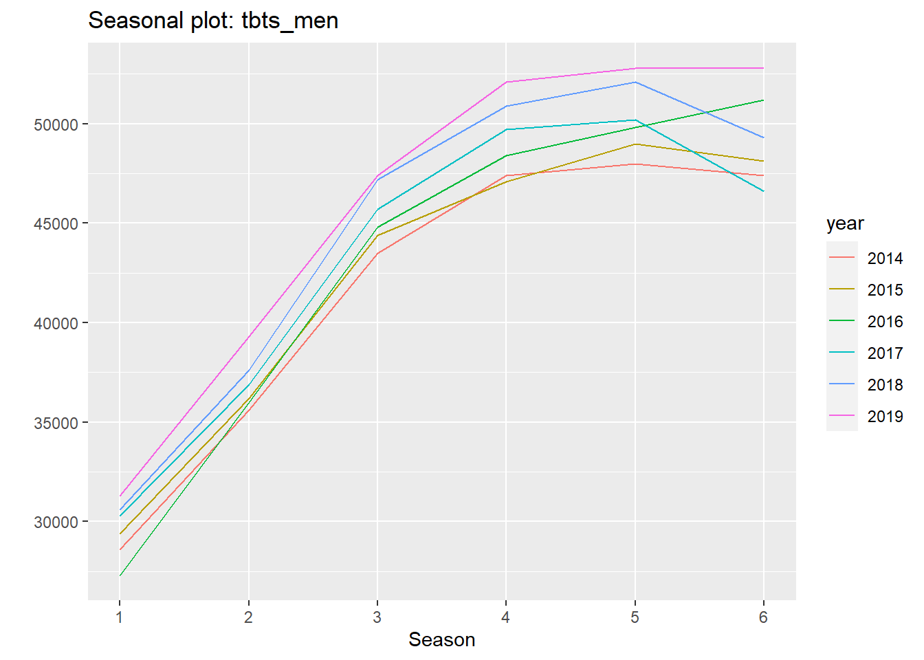
For women, the auto.arima is not able to pick up any SAR. The best fit is according to auto.arima is a constant drift.
arimamodel_women <- auto.arima(tbts_women)

summary(arimamodel_women)
## Series: tbts_women
## ARIMA(0,0,0)(0,1,0)[5] with drift
##
## Coefficients:
##          drift
##       188.0000
## s.e.   43.5542
##
## sigma^2 estimated as 1235313:  log likelihood=-210.3
## AIC=424.59   AICc=425.14   BIC=427.03
##
## Training set error measures:
##                    ME    RMSE     MAE         MPE     MAPE      MASE
## Training set 6.362663 994.108 699.696 -0.07692376 1.730501 0.6551461
##                     ACF1
## Training set -0.07256362

checkresiduals(arimamodel_women)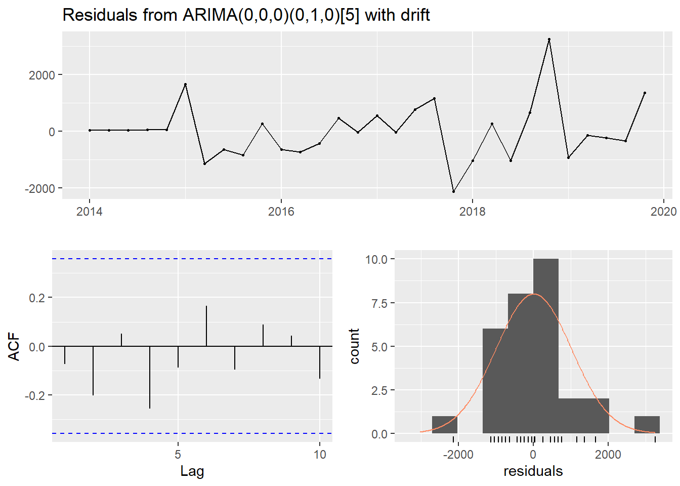
##
##  Ljung-Box test
##
## data:  Residuals from ARIMA(0,0,0)(0,1,0)[5] with drift
## Q* = 5.4793, df = 5, p-value = 0.3602
##
## Model df: 1.   Total lags used: 6

ggseasonplot(tbts_women)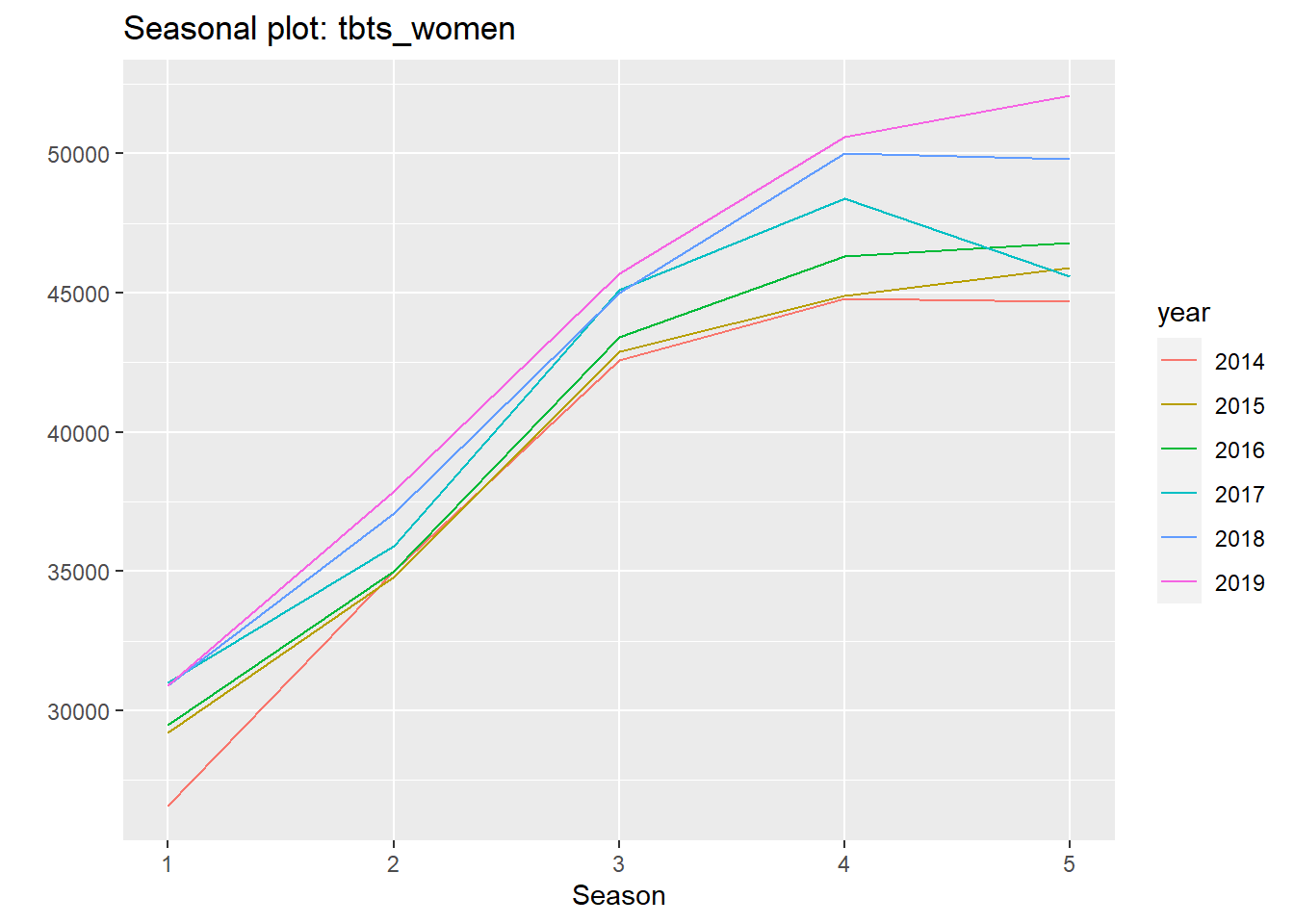
An AR(p) model assumes that a time series Yt can be modelled by a linear function of the first p of its lagged values. Let’s first start to model a seasonal SAR(1) model with the dynlm package. Each year the salaries increase by a fixed amount and a part that is relative to the salary size. I will use the NeweyWest function from the Sandwich package throughout this post to get heteroskedasticity- and autocorrelation-consistent error estimates.
dynmodel_men <- dynlm(ts(salary) ~ L(ts(salary), 6), data = tb_men)

assess_model(dynmodel_men, time(tbts_men)[7:36], tb_men[7:36,], no_n = TRUE)
##
## Time series regression with "ts" data:
## Start = 7, End = 36
##
## Call:
## dynlm(formula = ts(salary) ~ L(ts(salary), 6), data = tb_men)
##
## Residuals:
##     Min      1Q  Median      3Q     Max
## -5517.7  -371.7    48.9   418.0  2600.3
##
## Coefficients:
##                   Estimate Std. Error t value Pr(>|t|)
## (Intercept)      4.339e+02  1.575e+03   0.275    0.785
## L(ts(salary), 6) 1.009e+00  3.608e-02  27.980   <2e-16 ***
## ---
## Signif. codes:  0 '***' 0.001 '**' 0.01 '*' 0.05 '.' 0.1 ' ' 1
##
## Residual standard error: 1522 on 28 degrees of freedom
## Multiple R-squared:  0.9655, Adjusted R-squared:  0.9642
## F-statistic: 782.9 on 1 and 28 DF,  p-value: < 2.2e-16
##
##
## t test of coefficients:
##
##                    Estimate Std. Error t value Pr(>|t|)
## (Intercept)      4.3389e+02 1.8030e+03  0.2406   0.8116
## L(ts(salary), 6) 1.0094e+00 4.3076e-02 23.4340   <2e-16 ***
## ---
## Signif. codes:  0 '***' 0.001 '**' 0.01 '*' 0.05 '.' 0.1 ' ' 1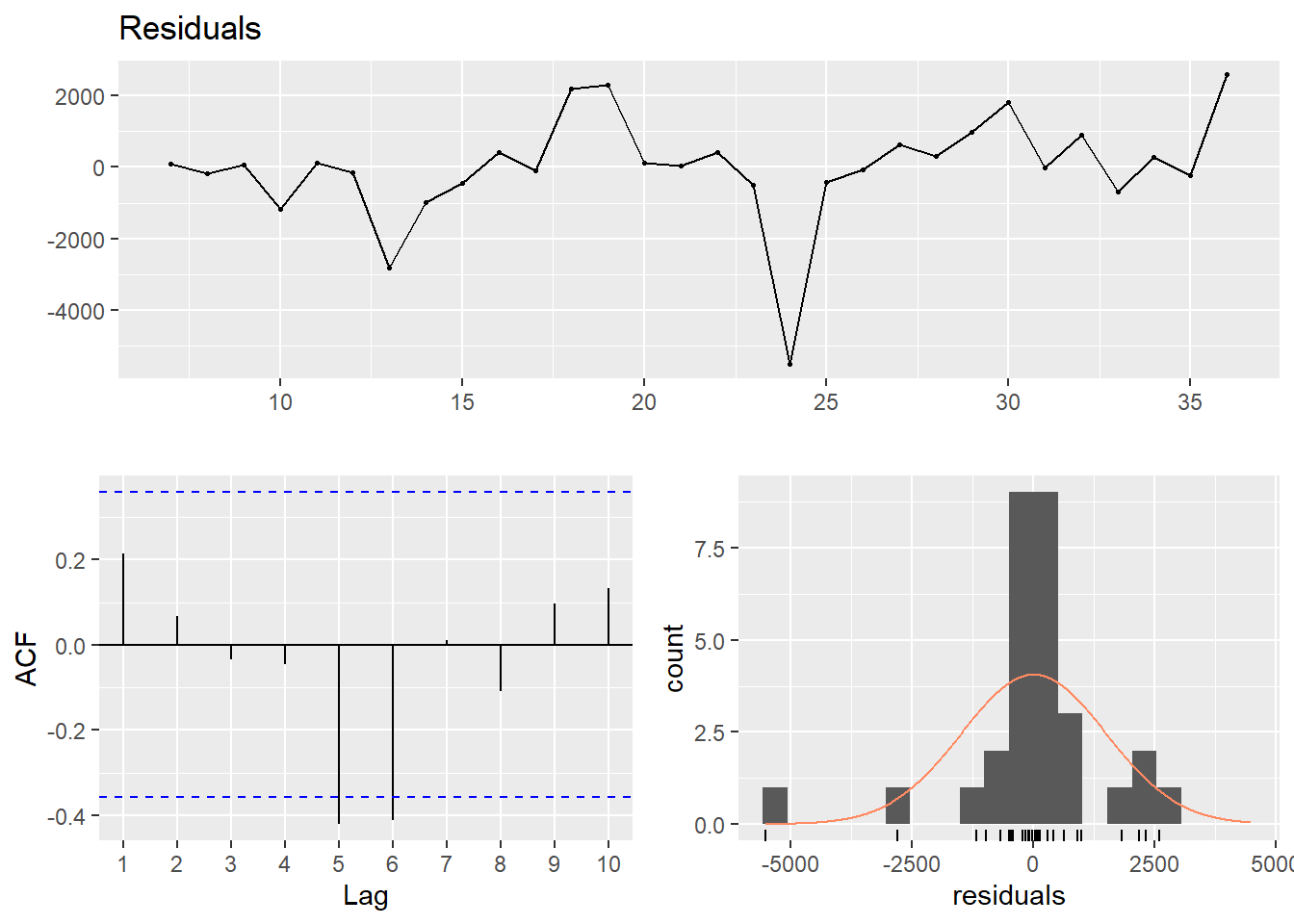
##
##  Breusch-Godfrey test for serial correlation of order up to 6
##
## data:  Residuals
## LM test = 9.8199, df = 6, p-value = 0.1324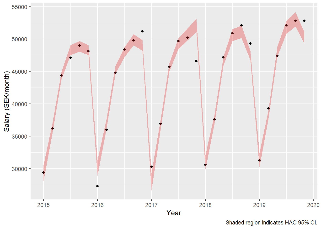
dynmodel_women <- dynlm(ts(salary) ~ L(ts(salary), 5), data = tb_women)

assess_model(dynmodel_women, time(tbts_women)[6:30], tb_women[6:30,], no_n = TRUE)
##
## Time series regression with "ts" data:
## Start = 6, End = 30
##
## Call:
## dynlm(formula = ts(salary) ~ L(ts(salary), 5), data = tb_women)
##
## Residuals:
##     Min      1Q  Median      3Q     Max
## -2266.8  -683.0  -148.9   501.2  3157.1
##
## Coefficients:
##                   Estimate Std. Error t value Pr(>|t|)
## (Intercept)      1.323e+02  1.316e+03   0.101    0.921
## L(ts(salary), 5) 1.020e+00  3.206e-02  31.816   <2e-16 ***
## ---
## Signif. codes:  0 '***' 0.001 '**' 0.01 '*' 0.05 '.' 0.1 ' ' 1
##
## Residual standard error: 1126 on 23 degrees of freedom
## Multiple R-squared:  0.9778, Adjusted R-squared:  0.9768
## F-statistic:  1012 on 1 and 23 DF,  p-value: < 2.2e-16
##
##
## t test of coefficients:
##
##                    Estimate Std. Error t value Pr(>|t|)
## (Intercept)      1.3234e+02 1.1458e+03  0.1155   0.9091
## L(ts(salary), 5) 1.0200e+00 2.9112e-02 35.0356   <2e-16 ***
## ---
## Signif. codes:  0 '***' 0.001 '**' 0.01 '*' 0.05 '.' 0.1 ' ' 1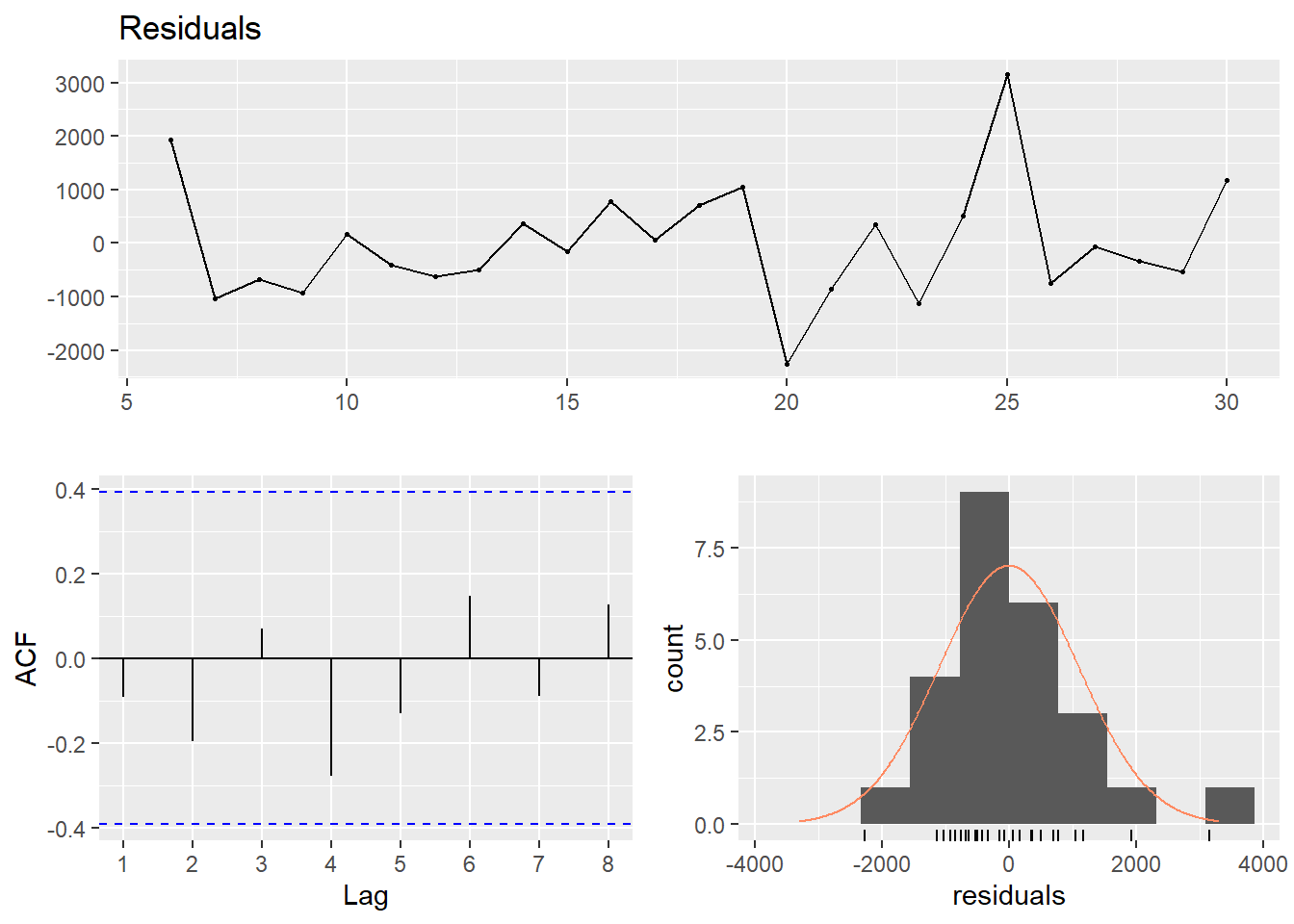
##
##  Breusch-Godfrey test for serial correlation of order up to 5
##
## data:  Residuals
## LM test = 4.8683, df = 5, p-value = 0.4322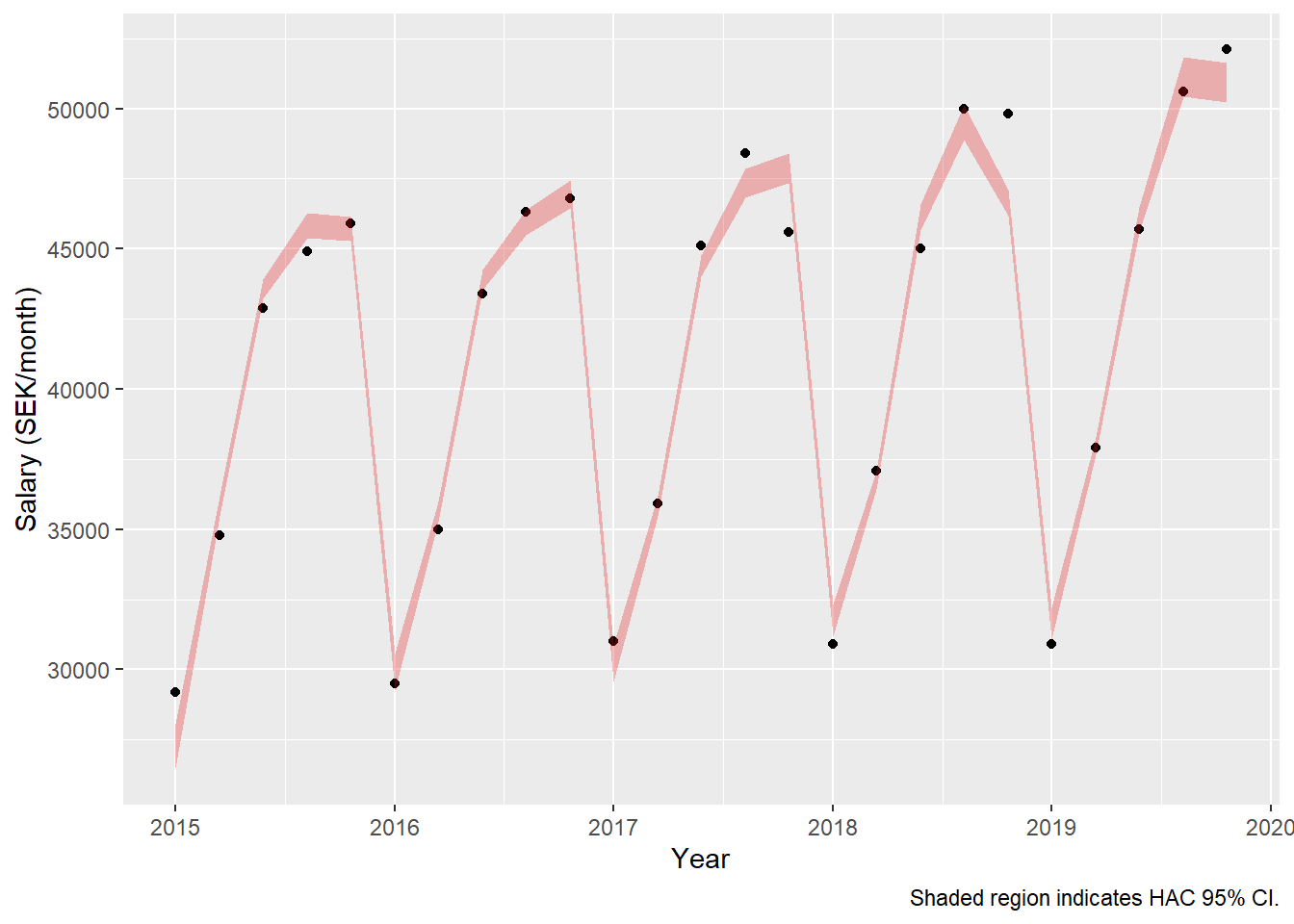
Now also add weights according to the number of engineers in the different strata. Note that the dynamic approach uses the information from the first year to predict the second. Weights from the first year have to be excluded. The fixed amount has decreased from 434 to 134 SEK and the relative part has increased from 0.94 % to 1.6 %. The fixed part is not statistically significant in either of these two models.
dynmodel_men <- dynlm(ts(salary) ~ L(ts(salary), 6), data = tb_men, weights = n[7:36])

assess_model(dynmodel_men, time(tbts_men)[7:36], tb_men[7:36,])
##
## Time series regression with "ts" data:
## Start = 7, End = 36
##
## Call:
## dynlm(formula = ts(salary) ~ L(ts(salary), 6), data = tb_men,
##     weights = n[7:36])
##
## Weighted Residuals:
##     Min      1Q  Median      3Q     Max
## -164527  -12301       0   48694  129992
##
## Coefficients:
##                   Estimate Std. Error t value Pr(>|t|)
## (Intercept)      1.343e+02  1.083e+03   0.124    0.902
## L(ts(salary), 6) 1.016e+00  2.398e-02  42.392   <2e-16 ***
## ---
## Signif. codes:  0 '***' 0.001 '**' 0.01 '*' 0.05 '.' 0.1 ' ' 1
##
## Residual standard error: 75460 on 21 degrees of freedom
## Multiple R-squared:  0.9884, Adjusted R-squared:  0.9879
## F-statistic:  1797 on 1 and 21 DF,  p-value: < 2.2e-16
##
##
## t test of coefficients:
##
##                   Estimate Std. Error t value Pr(>|t|)
## (Intercept)      134.30571  856.80707  0.1568   0.8769
## L(ts(salary), 6)   1.01643    0.01883 53.9780   <2e-16 ***
## ---
## Signif. codes:  0 '***' 0.001 '**' 0.01 '*' 0.05 '.' 0.1 ' ' 1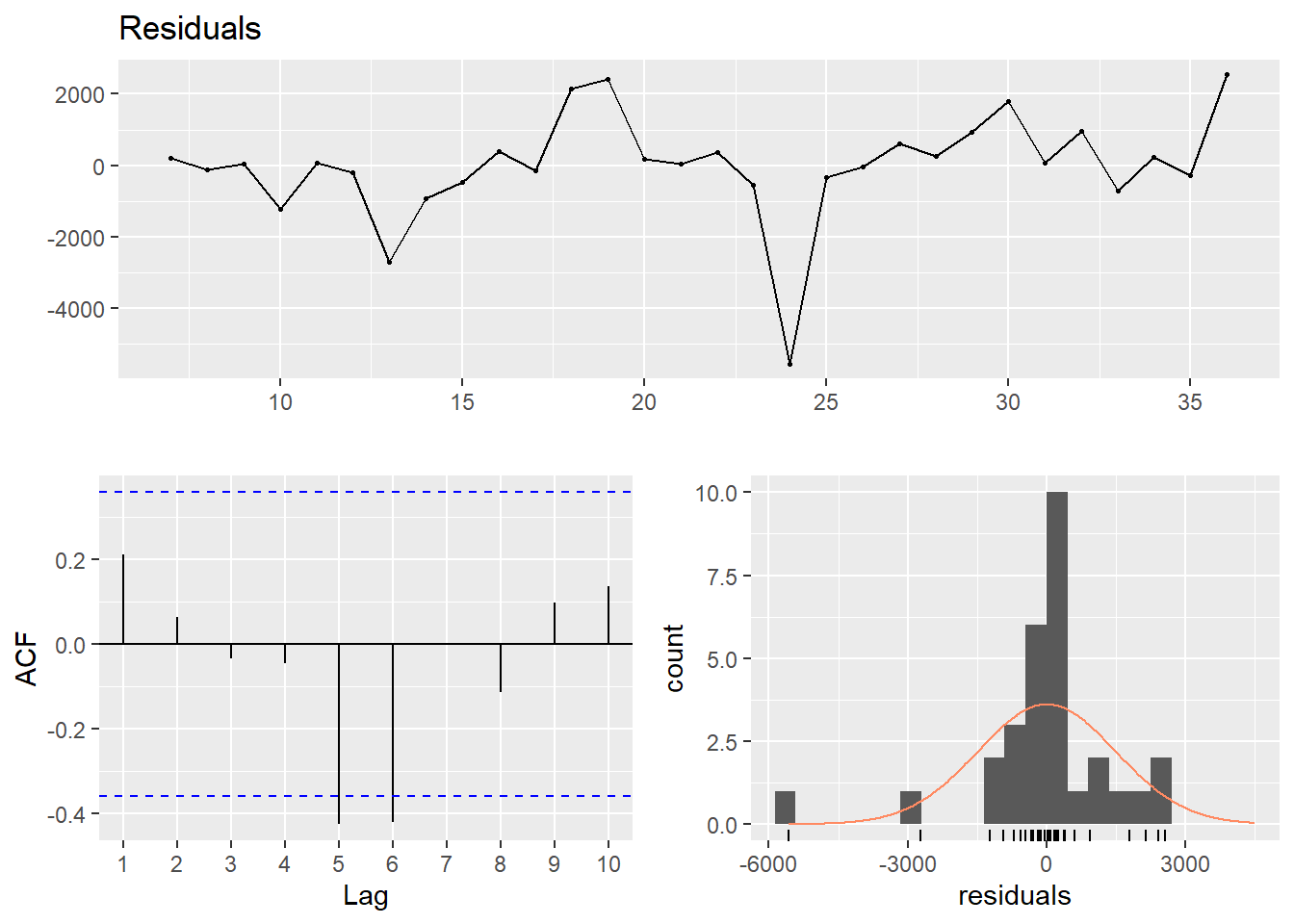
##
##  Breusch-Godfrey test for serial correlation of order up to 6
##
## data:  Residuals
## LM test = 9.8199, df = 6, p-value = 0.1324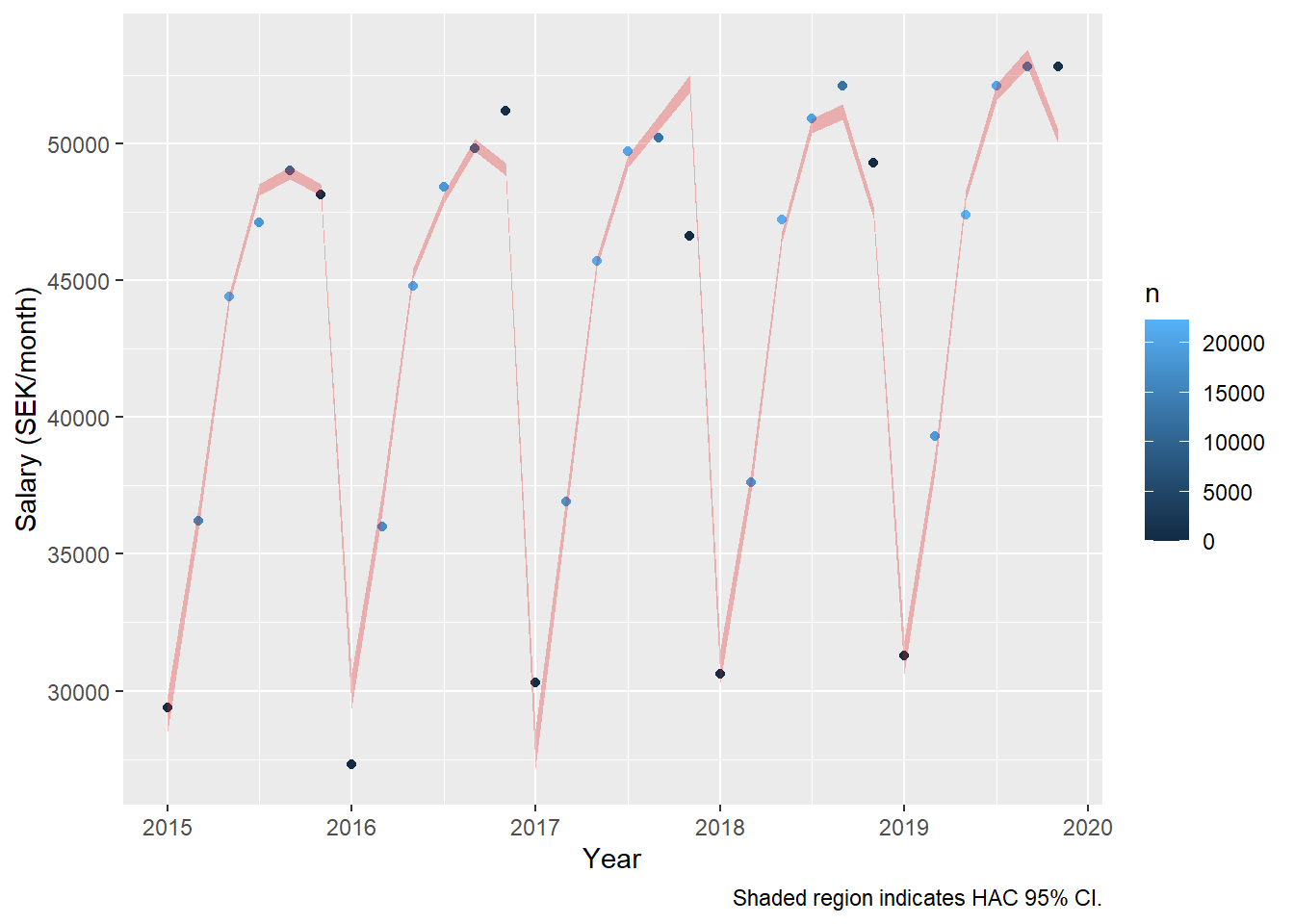
dynmodel_women <- dynlm(ts(salary) ~ L(ts(salary), 5), data = tb_women, weights = n[6:30])

assess_model(dynmodel_women, time(tbts_women)[6:30], tb_women[6:30,])
##
## Time series regression with "ts" data:
## Start = 6, End = 30
##
## Call:
## dynlm(formula = ts(salary) ~ L(ts(salary), 5), data = tb_women,
##     weights = n[6:30])
##
## Weighted Residuals:
##     Min      1Q  Median      3Q     Max
## -106359  -30874       0   33627  144325
##
## Coefficients:
##                    Estimate Std. Error t value Pr(>|t|)
## (Intercept)      -735.01210 1575.94230  -0.466    0.646
## L(ts(salary), 5)    1.03745    0.03693  28.089   <2e-16 ***
## ---
## Signif. codes:  0 '***' 0.001 '**' 0.01 '*' 0.05 '.' 0.1 ' ' 1
##
## Residual standard error: 60090 on 21 degrees of freedom
## Multiple R-squared:  0.9741, Adjusted R-squared:  0.9728
## F-statistic:   789 on 1 and 21 DF,  p-value: < 2.2e-16
##
##
## t test of coefficients:
##
##                     Estimate  Std. Error t value Pr(>|t|)
## (Intercept)      -735.012099  708.461714 -1.0375   0.3113
## L(ts(salary), 5)    1.037452    0.014893 69.6602   <2e-16 ***
## ---
## Signif. codes:  0 '***' 0.001 '**' 0.01 '*' 0.05 '.' 0.1 ' ' 1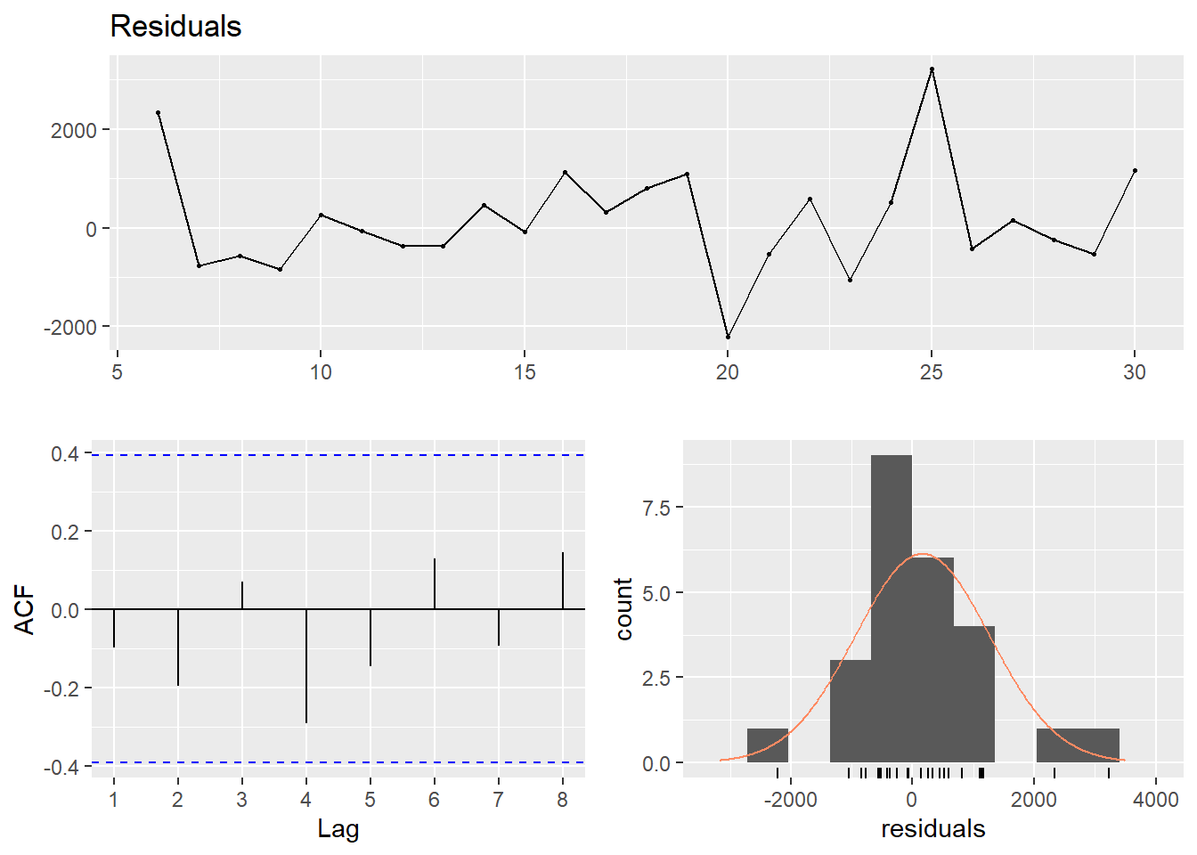
##
##  Breusch-Godfrey test for serial correlation of order up to 5
##
## data:  Residuals
## LM test = 4.8683, df = 5, p-value = 0.4322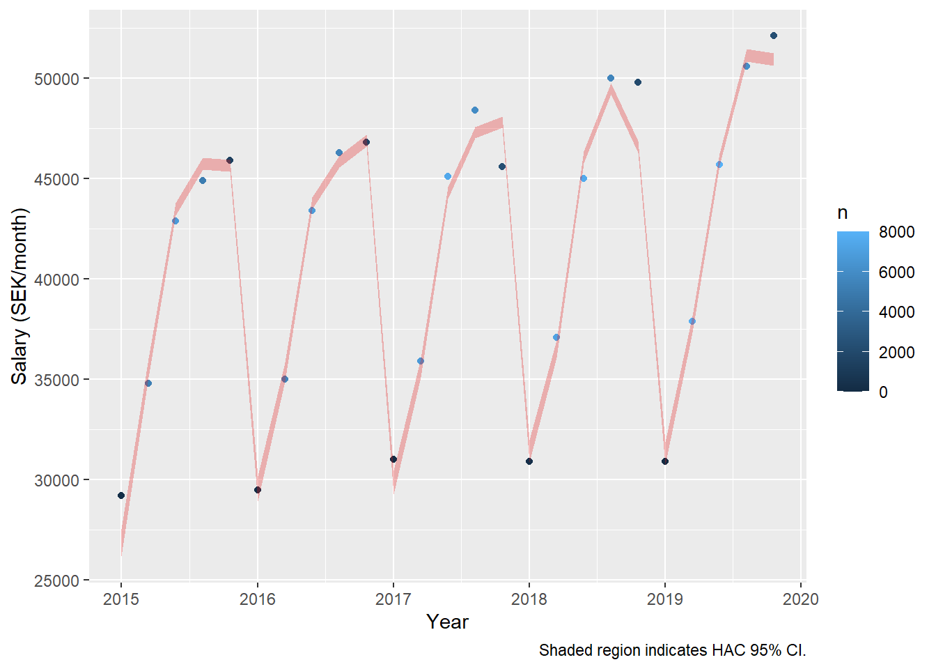
Let’s drop the non-significant intercept. The relative salary raise increases to 1,94 % per year for men and 2,03 % for women.
dynmodel_men <- dynlm(ts(salary) ~ L(ts(salary), 6) - 1, data = tb_men, weights = n[7:36])

assess_model(dynmodel_men, time(tbts_men)[7:36], tb_men[7:36,])
##
## Time series regression with "ts" data:
## Start = 7, End = 36
##
## Call:
## dynlm(formula = ts(salary) ~ L(ts(salary), 6) - 1, data = tb_men,
##     weights = n[7:36])
##
## Weighted Residuals:
##     Min      1Q  Median      3Q     Max
## -165299   -8902       0   47573  133181
##
## Coefficients:
##                  Estimate Std. Error t value Pr(>|t|)
## L(ts(salary), 6) 1.019380   0.002739   372.1   <2e-16 ***
## ---
## Signif. codes:  0 '***' 0.001 '**' 0.01 '*' 0.05 '.' 0.1 ' ' 1
##
## Residual standard error: 73750 on 22 degrees of freedom
## Multiple R-squared:  0.9998, Adjusted R-squared:  0.9998
## F-statistic: 1.385e+05 on 1 and 22 DF,  p-value: < 2.2e-16
##
##
## t test of coefficients:
##
##                   Estimate Std. Error t value  Pr(>|t|)
## L(ts(salary), 6) 1.0193798  0.0020172  505.35 < 2.2e-16 ***
## ---
## Signif. codes:  0 '***' 0.001 '**' 0.01 '*' 0.05 '.' 0.1 ' ' 1
##
##  Breusch-Godfrey test for serial correlation of order up to 6
##
## data:  Residuals
## LM test = 9.9529, df = 6, p-value = 0.1266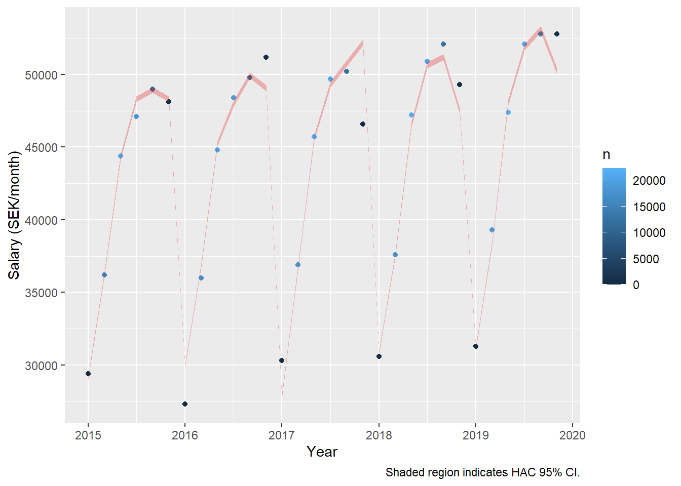
dynmodel_women <- dynlm(ts(salary) ~ L(ts(salary),5) - 1, data = tb_women, weights = n[6:30])

assess_model(dynmodel_women, time(tbts_women)[6:30], tb_women[6:30,])
##
## Time series regression with "ts" data:
## Start = 6, End = 30
##
## Call:
## dynlm(formula = ts(salary) ~ L(ts(salary), 5) - 1, data = tb_women,
##     weights = n[6:30])
##
## Weighted Residuals:
##     Min      1Q  Median      3Q     Max
## -103209  -32580       0   36088  146345
##
## Coefficients:
##                  Estimate Std. Error t value Pr(>|t|)
## L(ts(salary), 5) 1.020343   0.004217   241.9   <2e-16 ***
## ---
## Signif. codes:  0 '***' 0.001 '**' 0.01 '*' 0.05 '.' 0.1 ' ' 1
##
## Residual standard error: 59020 on 22 degrees of freedom
## Multiple R-squared:  0.9996, Adjusted R-squared:  0.9996
## F-statistic: 5.853e+04 on 1 and 22 DF,  p-value: < 2.2e-16
##
##
## t test of coefficients:
##
##                   Estimate Std. Error t value  Pr(>|t|)
## L(ts(salary), 5) 1.0203429  0.0035569  286.86 < 2.2e-16 ***
## ---
## Signif. codes:  0 '***' 0.001 '**' 0.01 '*' 0.05 '.' 0.1 ' ' 1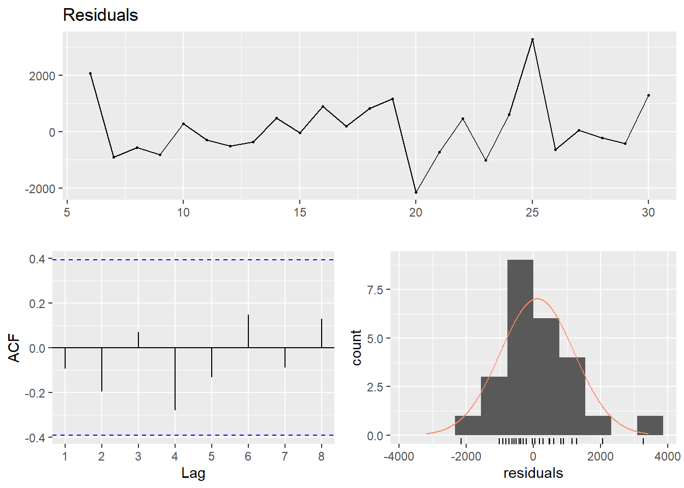
##
##  Breusch-Godfrey test for serial correlation of order up to 5
##
## data:  Residuals
## LM test = 4.9459, df = 5, p-value = 0.4225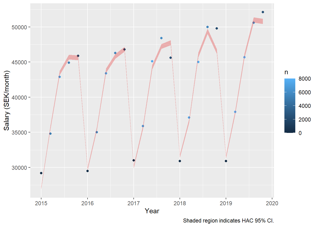
Now, let’s compare with a linear model. The relative salary raise increases to 1,92 % per year for men and 2.06 % for women.
model_men <- lm(log(salary) ~ year_n + age_n + I(age_n^2), data = tb_men, weights = n)

assess_model(model_men, time(tbts_men), tb_men, doexp = TRUE)
##
## Call:
## lm(formula = log(salary) ~ year_n + age_n + I(age_n^2), data = tb_men,
##     weights = n)
##
## Weighted Residuals:
##     Min      1Q  Median      3Q     Max
## -3.5386 -0.1234  0.0000  0.7387  2.7634
##
## Coefficients:
##               Estimate Std. Error t value Pr(>|t|)
## (Intercept) -2.925e+01  3.086e+00  -9.479 2.08e-09 ***
## year_n       1.917e-02  1.530e-03  12.534 9.23e-12 ***
## age_n        5.160e-02  2.286e-03  22.569  < 2e-16 ***
## I(age_n^2)  -4.670e-04  2.581e-05 -18.094 4.24e-15 ***
## ---
## Signif. codes:  0 '***' 0.001 '**' 0.01 '*' 0.05 '.' 0.1 ' ' 1
##
## Residual standard error: 1.694 on 23 degrees of freedom
## Multiple R-squared:  0.9898, Adjusted R-squared:  0.9885
## F-statistic: 746.4 on 3 and 23 DF,  p-value: < 2.2e-16
##
##
## t test of coefficients:
##
##                Estimate  Std. Error t value  Pr(>|t|)
## (Intercept) -2.9252e+01  1.8119e+00 -16.145 4.852e-14 ***
## year_n       1.9171e-02  9.0239e-04  21.244 < 2.2e-16 ***
## age_n        5.1595e-02  1.6460e-03  31.347 < 2.2e-16 ***
## I(age_n^2)  -4.6705e-04  1.7897e-05 -26.097 < 2.2e-16 ***
## ---
## Signif. codes:  0 '***' 0.001 '**' 0.01 '*' 0.05 '.' 0.1 ' ' 1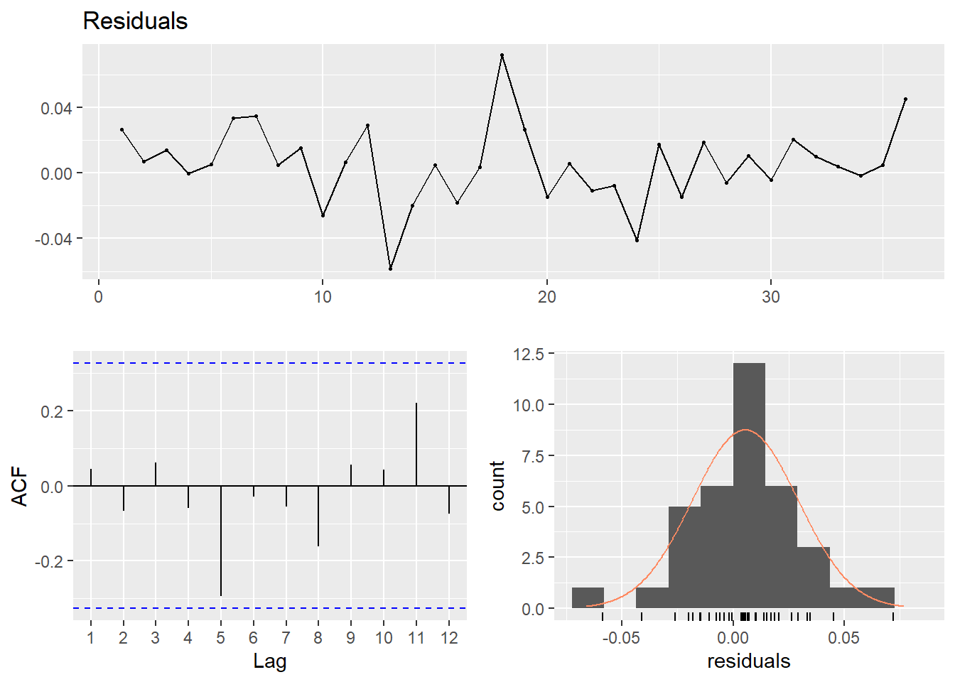
##
##  Breusch-Godfrey test for serial correlation of order up to 7
##
## data:  Residuals
## LM test = 6.7232, df = 7, p-value = 0.4583
## Don't know how to automatically pick scale for object of type ts. Defaulting to continuous.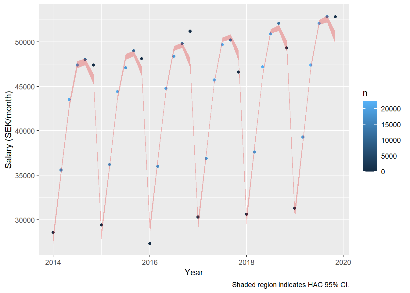
model_women <- lm(log(salary) ~ year_n + age_n + I(age_n^2), data = tb_women, weights = n)

assess_model(model_women, time(tbts_women), tb_women, doexp = TRUE)
##
## Call:
## lm(formula = log(salary) ~ year_n + age_n + I(age_n^2), data = tb_women,
##     weights = n)
##
## Weighted Residuals:
##      Min       1Q   Median       3Q      Max
## -2.31829 -0.34720  0.05136  0.89951  2.33846
##
## Coefficients:
##               Estimate Std. Error t value Pr(>|t|)
## (Intercept) -3.228e+01  4.347e+00  -7.427 1.50e-07 ***
## year_n       2.063e-02  2.154e-03   9.580 1.71e-09 ***
## age_n        5.521e-02  3.330e-03  16.577 2.77e-14 ***
## I(age_n^2)  -5.202e-04  3.912e-05 -13.298 2.77e-12 ***
## ---
## Signif. codes:  0 '***' 0.001 '**' 0.01 '*' 0.05 '.' 0.1 ' ' 1
##
## Residual standard error: 1.288 on 23 degrees of freedom
## Multiple R-squared:  0.9798, Adjusted R-squared:  0.9771
## F-statistic: 371.4 on 3 and 23 DF,  p-value: < 2.2e-16
##
##
## t test of coefficients:
##
##                Estimate  Std. Error  t value  Pr(>|t|)
## (Intercept) -3.2285e+01  3.9562e+00  -8.1605 3.045e-08 ***
## year_n       2.0631e-02  1.9667e-03  10.4903 3.075e-10 ***
## age_n        5.5206e-02  2.7439e-03  20.1196 4.246e-16 ***
## I(age_n^2)  -5.2025e-04  3.3832e-05 -15.3777 1.357e-13 ***
## ---
## Signif. codes:  0 '***' 0.001 '**' 0.01 '*' 0.05 '.' 0.1 ' ' 1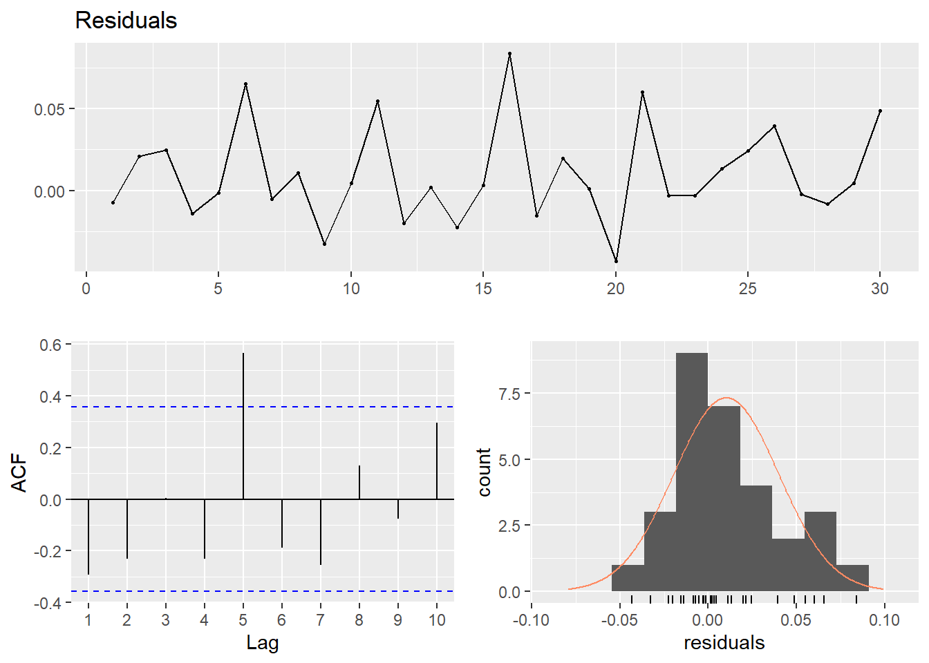
##
##  Breusch-Godfrey test for serial correlation of order up to 7
##
## data:  Residuals
## LM test = 11.678, df = 7, p-value = 0.1117
## Don't know how to automatically pick scale for object of type ts. Defaulting to continuous.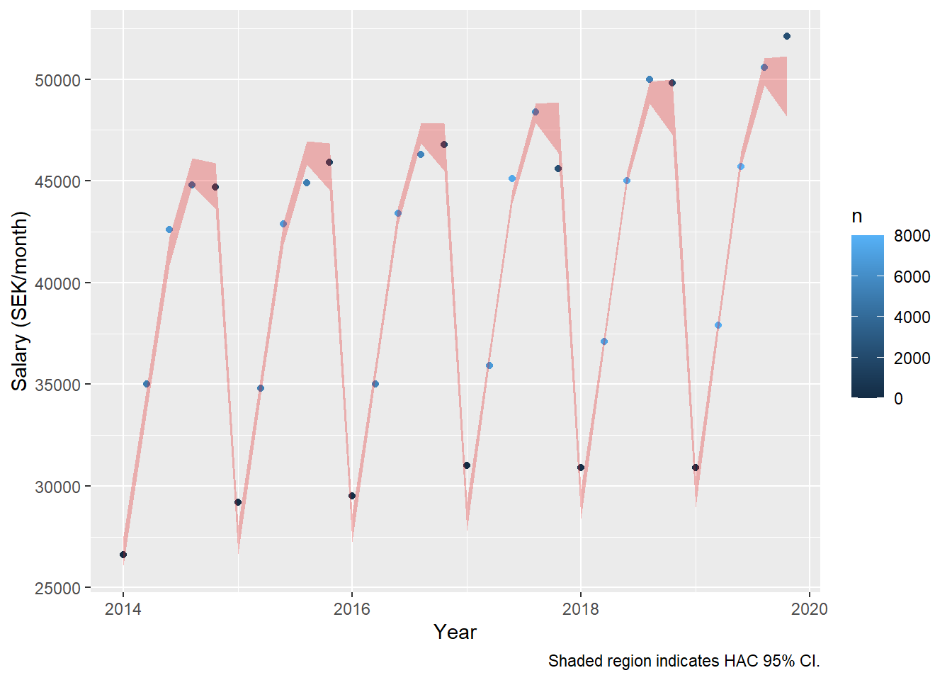
Now also add the SAR(2). The summary shows that the R-squared bumps up a few notches for men, although it does not show that the second year lag is significant. However, the sandwich package assures us that the SAR(2) process is significant at the 95 % level. For women, the second year lag is not significant in the summary nor the HAC error estimate.
dynmodel_men <- dynlm(ts(salary) ~ L(ts(salary), 6) + L(ts(salary), 12) - 1, data = tb_men, weights = n[13:36])

assess_model(dynmodel_men, time(tbts_men)[13:36], tb_men[13:36,])
##
## Time series regression with "ts" data:
## Start = 13, End = 36
##
## Call:
## dynlm(formula = ts(salary) ~ L(ts(salary), 6) + L(ts(salary),
##     12) - 1, data = tb_men, weights = n[13:36])
##
## Weighted Residuals:
##     Min      1Q  Median      3Q     Max
## -127942  -17989       0   42788  123721
##
## Coefficients:
##                   Estimate Std. Error t value Pr(>|t|)
## L(ts(salary), 6)    0.7282     0.2371   3.071  0.00692 **
## L(ts(salary), 12)   0.2985     0.2417   1.235  0.23356
## ---
## Signif. codes:  0 '***' 0.001 '**' 0.01 '*' 0.05 '.' 0.1 ' ' 1
##
## Residual standard error: 69840 on 17 degrees of freedom
## Multiple R-squared:  0.9999, Adjusted R-squared:  0.9999
## F-statistic: 6.4e+04 on 2 and 17 DF,  p-value: < 2.2e-16
##
##
## t test of coefficients:
##
##                   Estimate Std. Error t value  Pr(>|t|)
## L(ts(salary), 6)   0.72822    0.11497  6.3338 7.484e-06 ***
## L(ts(salary), 12)  0.29855    0.11741  2.5427   0.02102 *
## ---
## Signif. codes:  0 '***' 0.001 '**' 0.01 '*' 0.05 '.' 0.1 ' ' 1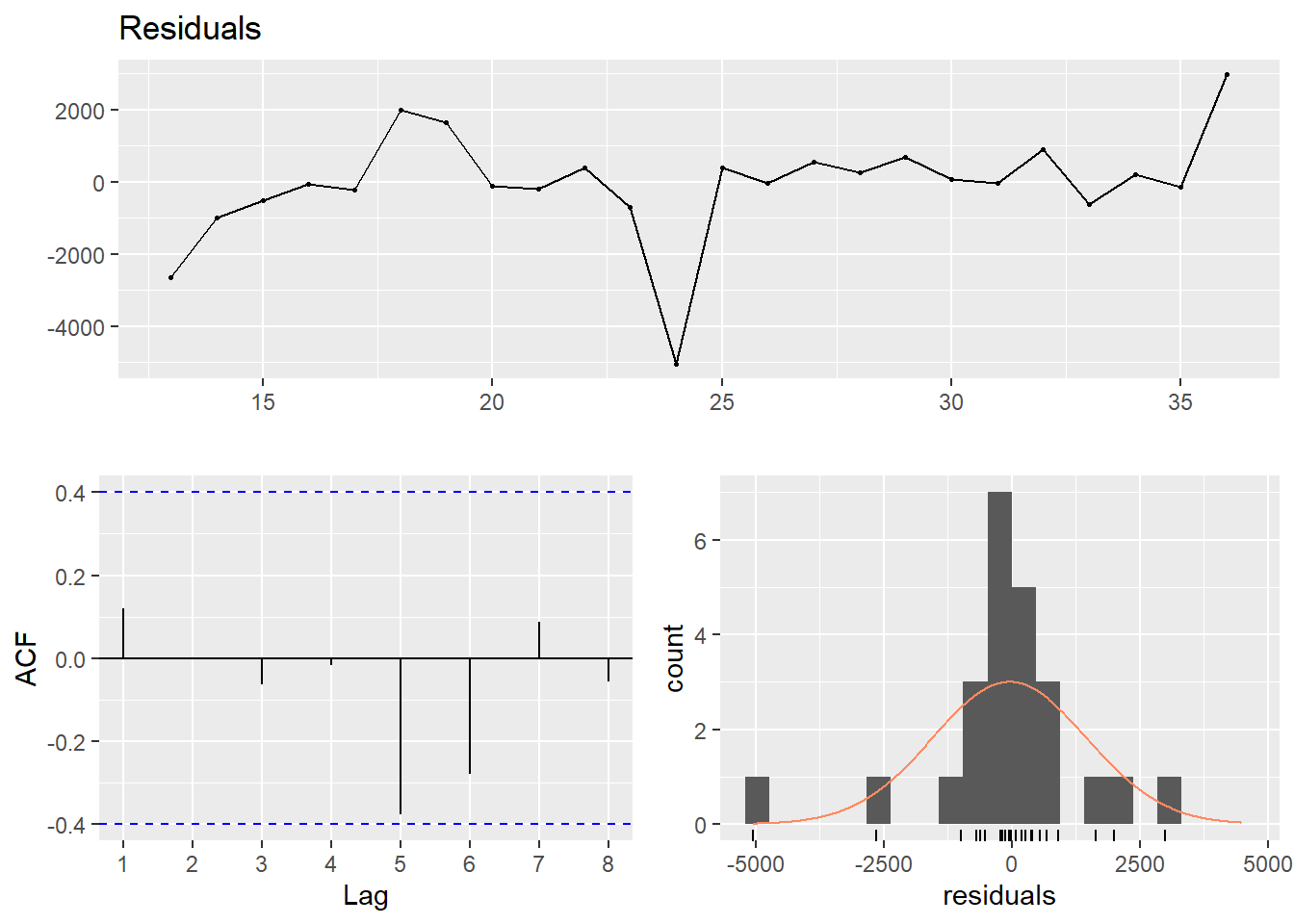
##
##  Breusch-Godfrey test for serial correlation of order up to 5
##
## data:  Residuals
## LM test = 3.9255, df = 5, p-value = 0.5602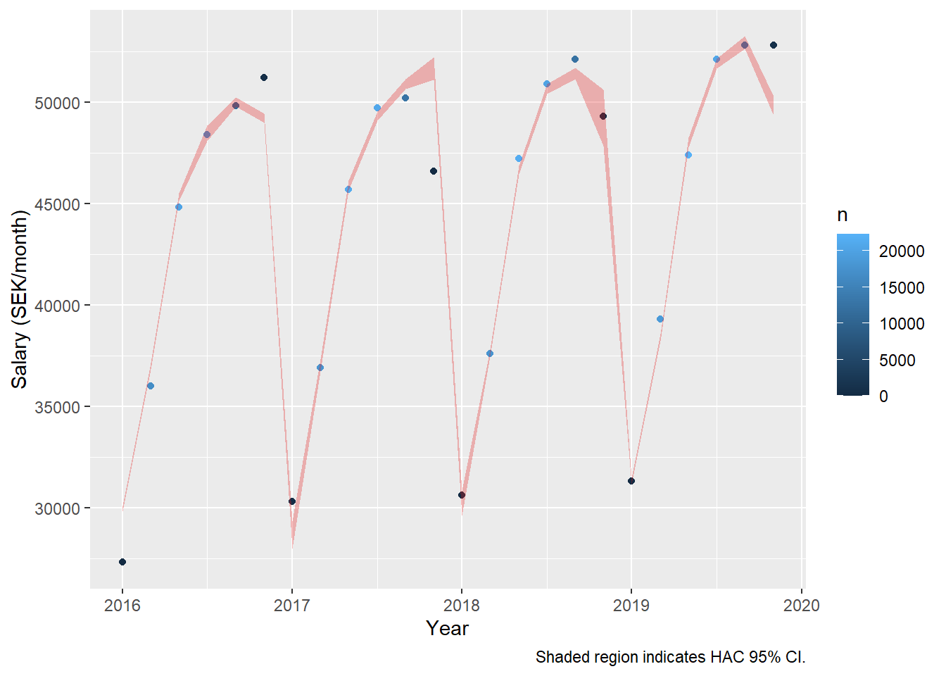
dynmodel_women <- dynlm(ts(salary) ~ L(ts(salary), 5) + L(ts(salary), 10) - 1, data = tb_women, weights = n[11:30])

summary (dynmodel_women)
##
## Time series regression with "ts" data:
## Start = 11, End = 30
##
## Call:
## dynlm(formula = ts(salary) ~ L(ts(salary), 5) + L(ts(salary),
##     10) - 1, data = tb_women, weights = n[11:30])
##
## Weighted Residuals:
##     Min      1Q  Median      3Q     Max
## -110096  -37862   -1787   33549  134747
##
## Coefficients:
##                   Estimate Std. Error t value Pr(>|t|)
## L(ts(salary), 5)   0.96703    0.23193   4.169 0.000723 ***
## L(ts(salary), 10)  0.05749    0.23683   0.243 0.811298
## ---
## Signif. codes:  0 '***' 0.001 '**' 0.01 '*' 0.05 '.' 0.1 ' ' 1
##
## Residual standard error: 63340 on 16 degrees of freedom
## Multiple R-squared:  0.9996, Adjusted R-squared:  0.9996
## F-statistic: 2.14e+04 on 2 and 16 DF,  p-value: < 2.2e-16

coeftest(dynmodel_women, vcov = NeweyWest, prewhite = F, adjust = T)
##
## t test of coefficients:
##
##                   Estimate Std. Error t value  Pr(>|t|)
## L(ts(salary), 5)  0.967032   0.122156  7.9164 6.354e-07 ***
## L(ts(salary), 10) 0.057485   0.125308  0.4588    0.6526
## ---
## Signif. codes:  0 '***' 0.001 '**' 0.01 '*' 0.05 '.' 0.1 ' ' 1